- / -
EMSC3025/6025: Remote Sensing of Water Resources

Aquifers
EMSC3025/6025
Dr. Sia Ghelichkhan
Objectives
By the end of this lecture, you should be able to:
Aquifer Classification:
- Define aquifers as the fundamental unit of groundwater hydrology
- Distinguish between unconfined, confined, and perched aquifers
- Classify confining beds: aquifuge, aquiclude, aquitard, and real-world aquitardifers
Aquifer Properties:
- Calculate transmissivity (
T = Kb ) and storativity (S ) - Explain specific storage, specific yield, and specific retention
- Compare storage mechanisms in confined vs unconfined aquifers
Objectives
By the end of this lecture, you should be able to:
Aquifer Systems:
- Identify major aquifer types: alluvial, fluvial, semiconsolidated, sandstone, carbonate-rock, fractured-rock and volcanic aquifers
- Understand how depositional environments control aquifer properties
- Recognise karst features: sinkholes, solution conduits, and cave systems
- Apply these concepts to Australia’s groundwater provinces, from the Great Artesian Basin to the Perth Basin and the Northern Territory carbonates
Introduction
- Just as the catchment is the basic unit of surface hydrology, the aquifer is the fundamental unit of groundwater hydrology.
- Aquifers are defined by their hydraulic properties rather than strictly by geology.
- Understanding aquifer types and properties is crucial for:
- Groundwater management
- Well design and sustainability
- Resource assessment
Key concept
An aquifer’s definition depends on context—what’s considered an aquifer in one region might be a confining bed in another.
Defining an Aquifer
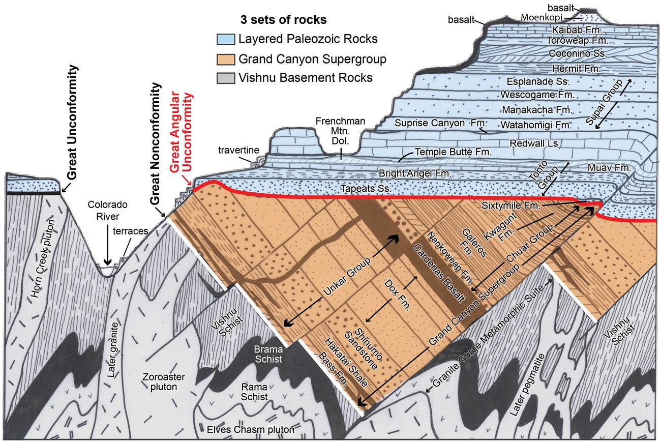
An aquifer is “a lithologic unit or combination of lithologic units capable of yielding water to pumped wells or springs”
— Domenico (1972)
- An aquifer can be:
- Coextensive with geologic formations
- A group of formations
- Part of a formation
- Independent of geologic units (cutting across formations)
Confining Beds
- Units of low permeability that bound an aquifer are called confining beds.
- The designation is context-dependent:
- In areas with prolific aquifers → low permeability unit = confining bed
- In groundwater-poor regions → same deposit might be considered an aquifer
Important note
In practice, this ambiguity is resolved by explicitly defining hydraulic conductivity or porosity values that characterise the unit. 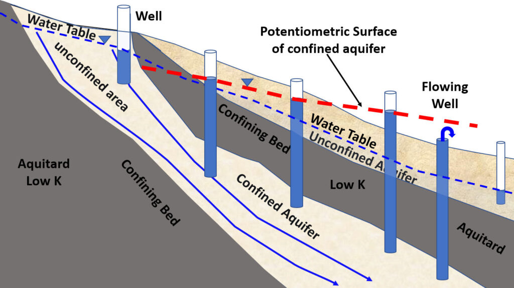
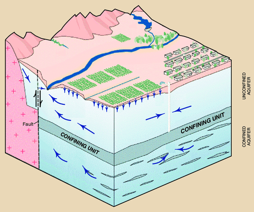
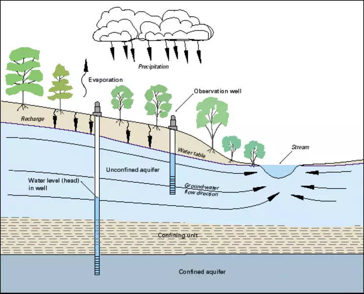
Unconfined Aquifers
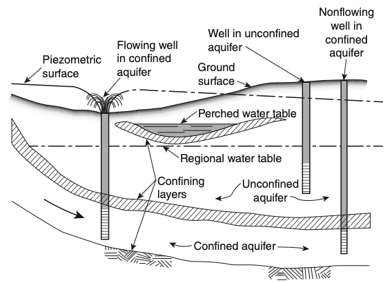
- Also called water table aquifers
- The water table forms the upper boundary
- No confining layer above
- Wells or piezometers installed in unconfined aquifers approximately define the water table position
- Water is under atmospheric pressure at the water table
Confined Aquifers
- Also called artesian aquifers
- Bounded by confining beds on both top and bottom
- Water is under pressure greater than atmospheric
- The water level in a well occurs above the upper boundary of the aquifer
- Occasionally, water level occurs above ground surface (flowing artesian well)
Perched Aquifers
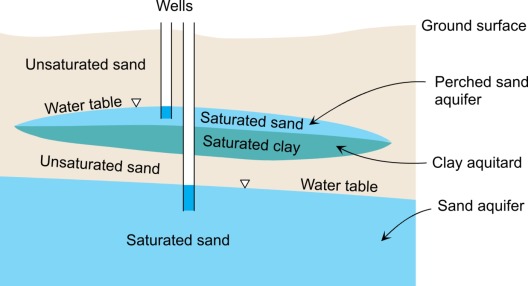
- An unconfined aquifer that develops above the regional water table
- Forms on top of a low hydraulic conductivity layer
- An unsaturated zone exists below the perched aquifer
- Often temporary or seasonal
- Important for local water supply in some areas
Key feature: Unsaturated zone both above and below the perched zone
Comparing Aquifer Types
| Aquifer Type | Upper Boundary | Lower Boundary | Pressure | Water Level |
|---|---|---|---|---|
| Unconfined | Water table (free surface) | Confining bed or impermeable layer | Atmospheric at water table | At water table |
| Confined | Confining bed | Confining bed | Above atmospheric | Above aquifer top |
| Perched | Water table | Low-K layer (perching layer) | Atmospheric at water table | Above regional water table |
Types of Confining Beds
Different Classifications of Confining Beds
Three terms are occasionally used to describe different types of confining beds:
Aquifuge
- The ultimate low hydraulic conductivity unit
- Extremely poor conductor of groundwater
- No storage capacity
- Example: intact unfractured crystalline rock
Aquiclude
- Similarly low permeability as aquifuge
- Able to store water (has porosity)
- Transmits water very slowly
- Example: clay layers
Aquitard
- A low permeability unit (leaky confining bed)
- Can store and transmit water between adjacent aquifers
- Stored water available to wells in nearby aquifers
- Example: silty clay layers
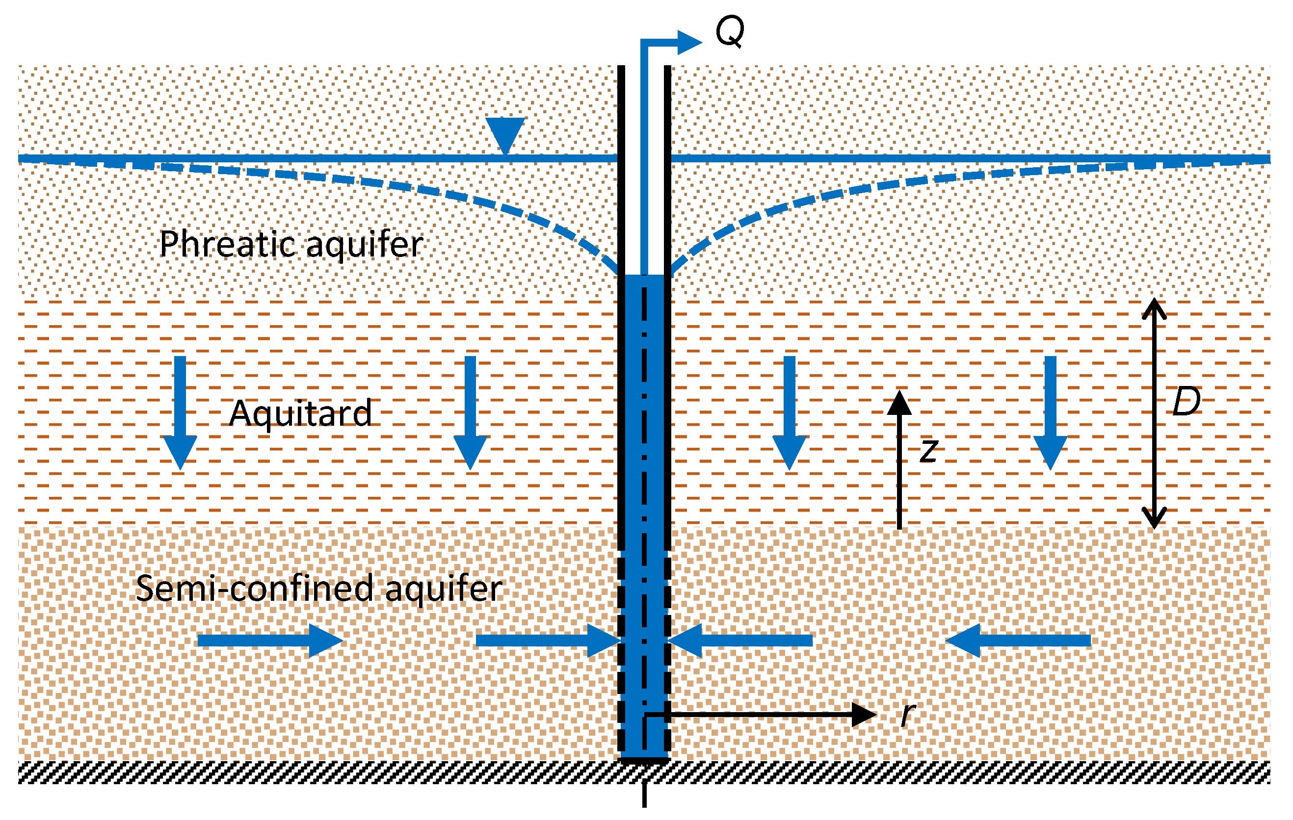
The Role of Aquitards
Aquitards play important dual roles:
- Influence rates of recharge between aquifer layers
- Can protect underlying aquifers from contaminants migrating downward from the ground surface
- Act as a barrier to vertical contaminant transport
- Provide slow release of water to adjacent aquifers during pumping
The Complexity of Real Aquitards
- Detailed characterisation in the midcontinent region of North America shows that simple concepts don’t capture reality.
- Runkel et al. (2018) use the term “aquitardifers” to describe confining beds that behave both as an aquitard and aquifer at the same place.
Key insight
Real confining beds are often more complex than simple one-dimensional models suggest.
Characteristics of Aquitardifers
Extreme anisotropy in hydraulic conductivity:
Horizontal direction:
- Permeable partings parallel to bedding
- Can transmit water horizontally like an aquifer
Vertical direction:
- Layering of low permeability units
- Sufficiently low
K_v to inhibit vertical transport of contaminants
Additional Complexity: Fractures
In some shallow settings, aquitardifers develop vertical fractures:
- Create fast-flow pathways
- Can extend over relatively large areas
- Provide direct connection between surface and deeper units
- Completely change the protective function of the confining bed
- Challenge simple predictions of contaminant transport
Management implication
Detailed site characterisation is essential—simple textbook models may not apply.
Key Aquifer Properties
Two Important Aquifer Properties
When a pump is turned on in a well:
- Water level in the well casing (and hydraulic head) is reduced
- This causes groundwater to flow from the aquifer into the well
- Much of the pumped water initially comes from “storage” in the aquifer
Therefore, aquifers have at least two important characteristics:
- Ability to store groundwater
- Ability to transmit this water to a nearby well
Key concept
These properties depend to an important extent on the geologic setting.
Transmissivity
Definition
The rate at which water of prevailing kinematic viscosity is transmitted through a unit width of the aquifer under a unit hydraulic gradient.
- Similar concept to hydraulic conductivity
- Main difference: applies across the vertical thickness of an aquifer
- Integrates conductivity over aquifer thickness
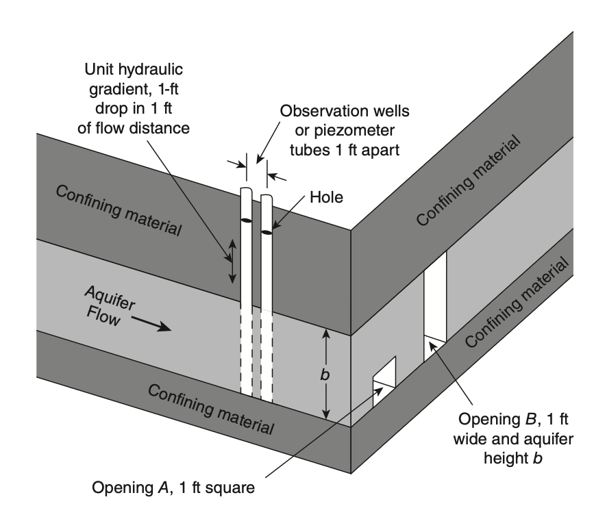
Transmissivity Equation
If the thickness of the aquifer is
Where:
T = transmissivity[L^2/T] K = hydraulic conductivity[L/T] b = aquifer thickness[L]
Units: m²/day, ft²/day, or gpd/ft (gallons per day per foot)
Physical meaning
Transmissivity tells you how much water can flow through the entire thickness of an aquifer per unit width.
Darcy’s Law for Aquifers
For a homogeneous confined aquifer, Darcy’s equation can be written in terms of transmissivity:
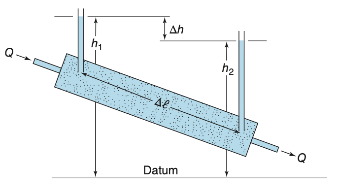
Apply Darcy’s law across the aquifer:
Where:
Q = discharge [L^3/T ]T = transmissivity [L^2/T ]W = width perpendicular to flow [L ]i = hydraulic gradient [dimensionless]
Storativity and Specific Storage
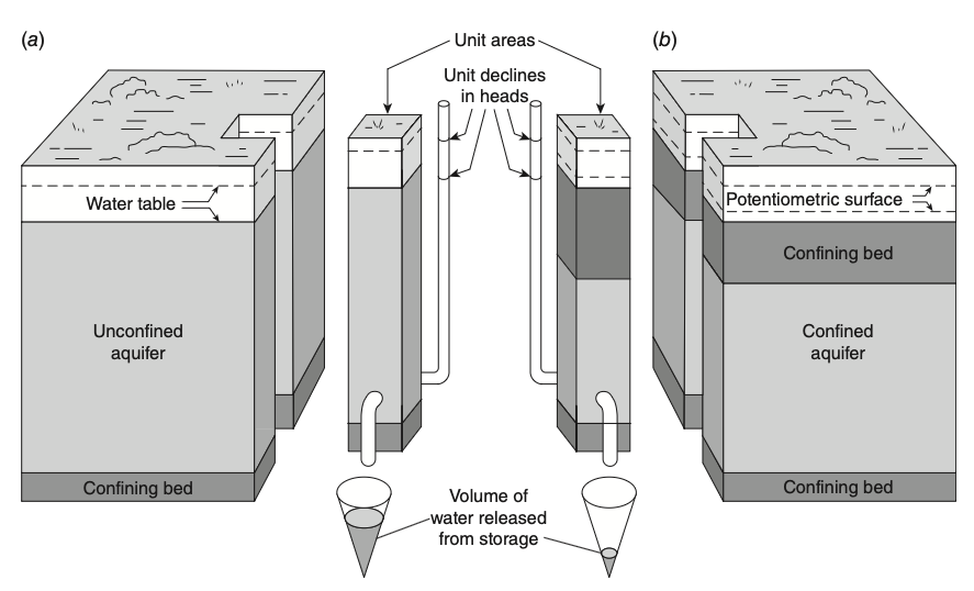
Aquifers can store water. How this storage is accomplished differs depending upon whether the aquifer is confined or unconfined.
Confined aquifer — Two mechanisms supply water:
- Water expansion: Lower pressure → water molecules expand slightly
- Aquifer compression: Lower water pressure → less support for skeleton → grains pushed closer together → squeezes water out
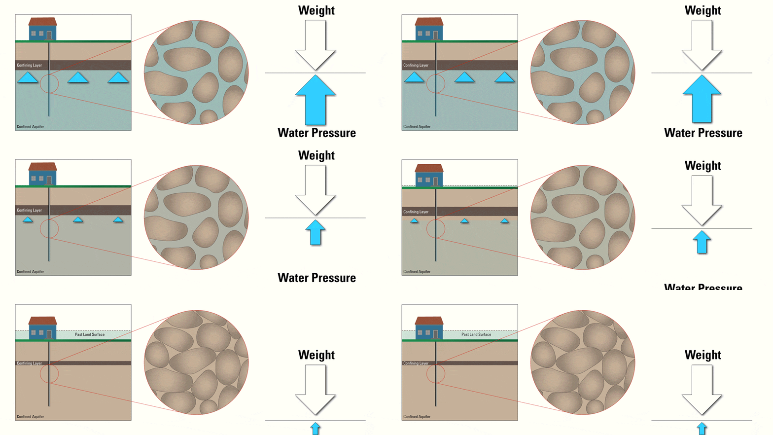
Understanding Aquifer Compression
Before pumping:
- Water pressure holds grains apart
- Aquifer skeleton is supported
- Pore space is at maximum
During pumping (head declines):
- Water pressure decreases
- Weight of overlying rocks pushes down
- Grains move closer together
- Pore space reduces → water squeezed out
Result: Only small amounts of water released (
Land Subsidence: Permanent Compression
When pumping is excessive or prolonged:
- Initial compression is elastic (recoverable)
- Continued compression becomes plastic (permanent)
- Aquifer structure permanently altered
- Land surface subsides
Why clay layers are critical:
- Clay is ~1000× more compressible than rock
- Major contributor to subsidence
- Once compressed, cannot recover
Real-world example
Latrobe Valley, Victoria:
- Open-cut coal mines pump the confined Latrobe Group aquifers
- Heads fell 120 to 130 m at the mines
- Land subsided 1 to 2.2 m near the mines, from compaction of coal and clay
Storage in Unconfined Aquifers
Unconfined aquifer:
- Main source of water is drainage of water from pores as the water table declines
- Much more water released per unit decline in head
- For a comparable unit decline in hydraulic head, an unconfined aquifer releases much more water from storage than a confined aquifer
Storativity Definition
Storativity (
- Dimensionless quantity
- For confined aquifers:
S ranges between10^{-3} to10^{-5} - For unconfined aquifers:
S (or specific yield) ranges between0.01 to0.30
Specific Storage
Specific storage (
Units:
Relationship between
where
Visual Summary: Storativity
Comparing Storage Properties
| Property | Symbol | Definition | Units | Typical Values |
|---|---|---|---|---|
| Specific Storage | Storage per unit volume | |||
| Storativity (confined) | Storage per unit area | Dimensionless | ||
| Specific Yield (unconfined) | Drainable porosity | Dimensionless |
Mathematical Formulation of Storage
Specific Storage from Compressibility
In a confined aquifer, specific storage comes from compression of the matrix and expansion of water (Domenico and Schwartz, 1998):
\rho_w g \approx 10^4 N/m³n = porosity\beta_p = vertical compressibility of the matrix\beta_w = 4.4 \times 10^{-10} m²/N = compressibility of water
Example: a clay with
| Material | Compressibility (m²/N) |
|---|---|
| Clay | |
| Sand | |
| Gravel | |
| Jointed rock | |
| Sound rock | |
| Water |
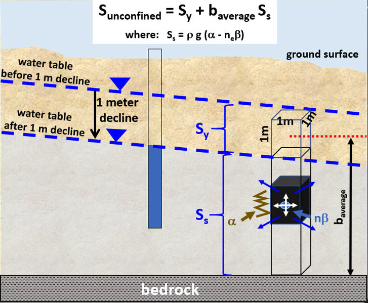
Storativity of Unconfined Aquifers
An unconfined aquifer releases water in two ways:
- Early time: expansion of water and compression of the matrix, as in a confined aquifer
- Later: gravity drainage of pores as the water table falls
S_y \approx 0.1 to0.3 bS_s \approx 10^{-5} to10^{-3} - So specific yield dominates in an unconfined aquifer
If pumping lowers the head below the top of a confined aquifer, the aquifer becomes unconfined and its storativity rises by several orders of magnitude.
Specific Yield and Specific Retention
Not all the water in the pores drains under gravity:
- Specific yield
S_y = V_d / V_T : the volume that drains by gravity, per total volume - Specific retention
S_r = V_r / V_T : the volume held as a film on grains and in small openings, per total volume
Specific retention increases as grain size and pore size decrease.
| Material | |
|---|---|
| Coarse gravel | 0.01 to 0.05 |
| Fine sand | 0.05 to 0.15 |
| Silt | 0.15 to 0.30 |
| Clay | 0.30 to 0.50 |
Clay has a high porosity, but most of its water is retained, so it yields little.
Types of Aquifer Systems
Unconsolidated Sand and Gravel Aquifers
Characteristics:
- Intergranular porosity
- Primarily unconfined conditions
- High permeability (varies with clay content and sorting)
- The most heavily pumped aquifer type in Australia
Three main settings in Australia:
- Alluvial: the Lachlan, Namoi, Murrumbidgee and Condamine rivers, the Lockyer Valley
- Coastal sand: the superficial aquifer under Perth, the Burdekin delta
- Palaeovalley: sand buried in old river channels, for example under the Yilgarn
Key properties
- High storage and transmission
- Thicker deposits → more regional flow
- Susceptible to contamination
- Alluvial aquifers hold about 20% of Australia’s bores but give about 60% of the extraction
Valley-Fill, Palaeovalley and Fluvial Aquifers
Valley-Fill and Palaeovalley Aquifers:
- Sediment that fills a valley or a buried river channel
- Long, narrow bodies with interbedded materials
- Examples: the Condamine and Lockyer valleys (Qld)
- Yilgarn palaeochannel sands:
K = 20–70 m/day, water more than 100 000 years old
Fluvial Aquifers:
- Deposited by river systems
- Two types: meandering vs braided
- Braided → more continuous and productive
- Long, narrow, thin geometry
- High specific yield (
0.1-0.3 ) - Examples: the Shepparton and Calivil formations of the Murray–Darling rivers
Semiconsolidated and Consolidated Aquifers
Semiconsolidated Sediments:
- Layered sand, clay and limestone in young basins
- Coastal wedges thicken toward the sea: unconfined where they crop out, confined further down dip
- Examples: the Murray Basin, the Gippsland Basin, Bundaberg
- Risk: saltwater intrusion (Bundaberg, about 12 500 ha lost)
- Risk: land subsidence (Latrobe Valley, 1 to 2.2 m)
Sandstone Aquifers:
- Cemented sand with reduced porosity
- Flow in fractures and bedding planes
- Low to moderate hydraulic conductivity
- Large areal extent
- Example: the Great Artesian Basin, recharged on its eastern outcrop at about 15 mm/yr
Carbonate-Rock Aquifers:
- Limestone and dolostone
- Solution-enhanced permeability
- 10 orders of magnitude range in
K - Large yields where well-connected
- Examples: the Tindall Limestone (NT), the Gambier Limestone (SA)
Other Types:
- Crystalline-rock: fractured granite and metasediments, flow in fractures
- Volcanic-rock: basalt with cooling fractures and lava tubes
Carbonate Aquifer Characteristics
Composition:
- Calcite (CaCO₃) → limestone
- Dolomite (CaMg(CO₃)₂) → dolostone
- Marine origin (shells, corals, algae, precipitates)
Solution openings range from:
- Small tubes and widened joints
- To caverns tens of meters wide
- Extending hundreds to thousands of meters in length
Hydraulic properties:
- Well-connected networks → large yields to wells
- Undissolved rock between openings → nearly impermeable
- Extreme heterogeneity
Australian examples
The Tindall Limestone (NT), the Gambier Limestone (SA) and the Millstream dolomite (WA). Each has a slide in the Australian section, with measured transmissivities and spring flows.
Karst Systems Summary
Formation requirements:
- Chemically aggressive groundwater
- Fractures present for transmission
- Groundwater can drain out
Solution features:
- Start as small conduits (~1 cm)
- Grow to cave size (kilometers long)
- Highest yields at fracture intersections
- Extremely heterogeneous permeability
Karst landforms:
- Sinkholes (dissolution, cover subsidence, cover-collapse)
- Stream sinks (disappearing streams)
- Dry valleys
- Large spring systems
- Underground cave networks
Australian examples:
- The Nullarbor: the largest area of exposed karst in the world
- Mount Gambier: sinkholes and cenotes
- Mataranka springs (NT)
Other Important Aquifer Types
Crystalline-rock aquifers:
- Fractured granite, basalt, metamorphic rocks
- Very low primary porosity
- Flow occurs primarily in fractures
- Secondary porosity controls productivity
- Examples: the Yilgarn (WA), the Mount Lofty Ranges (SA), the eastern highlands
- Well yields highly variable
Volcanic-rock aquifers:
- Basalt flows with high permeability
- Flow in cooling fractures and lava tubes
- Vesicular zones store water
- Examples: the Newer Volcanics (Vic), the Atherton Tablelands (Qld)
- Can be extremely productive locally
- Complex interbedded structure
Comparing Major Aquifer Types
| Aquifer Type | Porosity | K Range | Storage | Key Feature | Main Challenge |
|---|---|---|---|---|---|
| Unconsolidated | High (0.25-0.35) | High | Intergranular | Contamination | |
| Valley-fill, palaeovalley | High | High-Moderate | High | Long, narrow bodies | Over-exploitation |
| Fluvial (braided) | High | High | High | Lateral continuity | Variable quality |
| Semiconsolidated | Moderate | Moderate | Moderate | Wedge geometry | Subsidence, saltwater |
| Sandstone | Low-Moderate | Low-Moderate | Fracture flow | Vertical leakage | |
| Carbonate | Variable | 10 orders of magnitude | Variable | Solution conduits | Heterogeneity |
| Karst | Highly variable | Extremely high locally | Low-Moderate | Caves and conduits | Rapid transport |
| Crystalline | Very low | Very low | Very low | Fractures only | Limited yield |
Comparison of principal aquifer characteristics
Australian Aquifer Systems
Groundwater in Australia
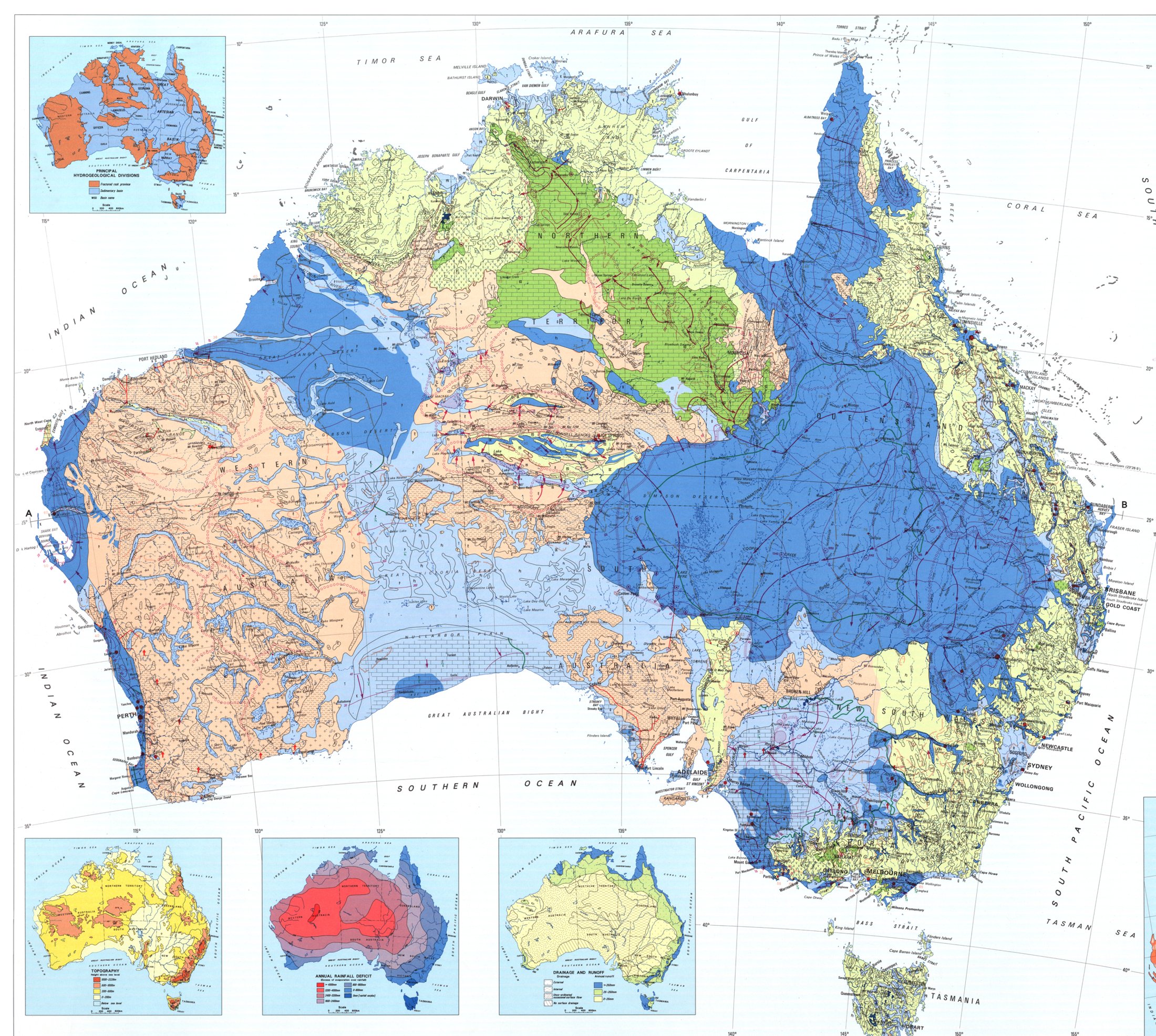
- Australia uses about 3 to 5 thousand GL of groundwater per year. The ABS counted 3,249 GL of self-extracted groundwater in 2021–22.
- Groundwater is about one fifth to one third of all water use. The share depends on the year and on how use is counted.
- Irrigation and stock take most of it, then mining, then town supply.
- The Northern Territory gets about 90% of its water from aquifers, and Western Australia about two thirds.
- In much of the arid interior, groundwater is the only reliable supply for towns, stations and mines.
Alluvial aquifers hold about 20% of all bores but give about 60% of the extraction.
How the aquifers are classified
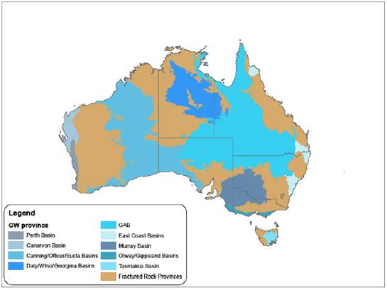
Three newer schemes use the same idea at different scales:
- Geoscience Australia uses six aquifer settings: alluvial, coastal, fractured rock, sedimentary basin, palaeovalley and karst.
- The National Hydrogeological Inventory (2023) splits the continent into about 40 groundwater provinces: sedimentary basins and fractured-rock provinces.
- The Bureau of Meteorology’s National Aquifer Framework groups formations into hydrogeologic units and complexes, so that every state uses the same names.
About 40% of Australia’s groundwater is stored in fractured rock, but fractured rock gives only about 10% of the extraction.
Great Artesian Basin
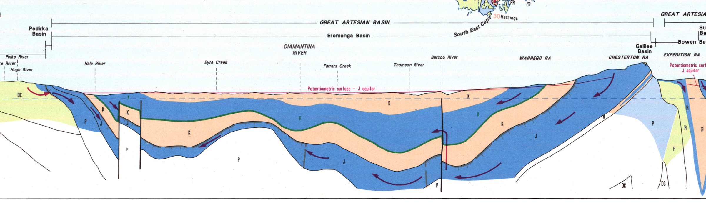
- More than 1.7 million km², one fifth of Australia (Qld, NSW, SA, NT).
- Jurassic–Cretaceous sandstones under the marine Rolling Downs mudstone. The basin fill is up to 3000 m thick.
- Confined and artesian.
K = 0.1 to 10 m/day,S \approx 10^{-5} .
- Recharge on the eastern outcrop, mean about 15 mm/yr.
- Flow 1 to 5 m/yr. Water near the centre is more than one million years old.
Great Artesian Basin: 140 years of flowing bores
Use: about 450 GL/yr. Stock 41%, irrigation 25%, oil and gas 19%, more than 120 towns 9%.
Pressure loss:
- About 4700 flowing bores were drilled after the 1880s.
- Open bore drains up to 100 km long lost more than 90% of the water to seepage and evaporation.
- Heads fell by up to about 100 m, and many springs stopped flowing.
Recovery:
- Bore capping and piping (GABSI, 1999–2017) controlled about 750 bores and replaced 21 000 km of drains.
- This saves about 250 GL/yr, and pressures are rising again in many areas.
Springs
More than 460 spring groups depend on GAB discharge. The mound springs near Lake Eyre are a listed endangered ecological community.
Coal seam gas
Gas wells in the Surat Basin pump about 52 GL/yr of water from coal seams. Drawdown in the Walloon Coal Measures is up to 280 m.
Murray Basin
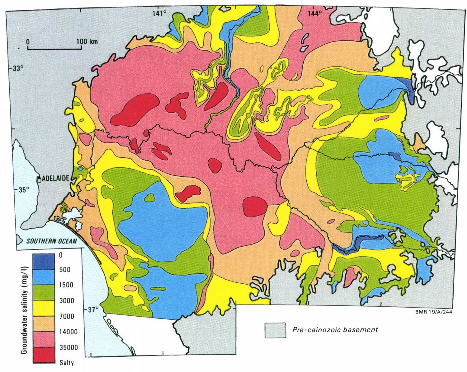
- A saucer-shaped Cenozoic basin of about 300 000 km² under NSW, Vic and SA, up to about 600 m thick.
- Stacked porous aquifers: the confined Renmark Group (fluvial sand), the Murray Group limestone, the Pliocene sands, and the Shepparton Formation at the top.
- A closed groundwater basin. The River Murray is the only drain for water and salt.
- Salinity ranges from below 200 to 300 000 mg/L.
Clearing the Mallee raised recharge from below 0.1 mm/yr to 8–40 mm/yr. Fourteen salt interception schemes now pump saline groundwater away from the river.
Alluvial aquifers of the Murray–Darling rivers
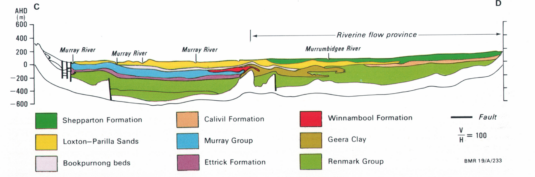
- Lachlan, Namoi, Murrumbidgee, Condamine: unconsolidated sand and gravel, unconfined over confined layers.
- Most recharge on the plains is leakage from rivers. Pumping turned many gaining rivers into losing rivers.
- Basin groundwater use: 1832 GL in 2004–05 (16% of all water use), 1232 GL in 2023–24.
- Lower Namoi in 2002: allocations of 213 GL/yr against a sustainable yield of 95 GL/yr. The limit is now 86 GL/yr. Condamine: levels down 3 to 35 m since the 1960s.
Perth Basin
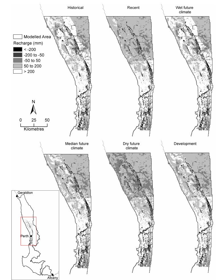
- A rift basin about 1300 km long. Fresh groundwater reaches about 1 km below Perth.
- Superficial aquifer: unconfined sand, with karstic Tamala Limestone at the coast (
K up to 100–1000 m/day). Recharge builds two water-table mounds, Gnangara and Jandakot. - Leederville and Yarragadee: deep, confined, layered sandstone, with water up to about 36 000 years old.
- Groundwater supplies about 70% of all water used in Perth and Mandurah.
Rainfall has fallen about 15% since 1975. The Gnangara Mound has lost more than 1000 GL of storage since 1980, and wetlands and cave pools have dried. Perth can now inject up to 28 GL/yr of recycled water into the confined aquifers.
Otway Basin: Mount Gambier
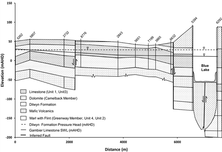
- Gambier Limestone: unconfined karst, with sinkholes, cenotes and spring-fed ponds.
T = 450 to 24 000 m²/day. - Dilwyn Formation: confined sand below, artesian in places. Most of its water is older than 25 000 years.
- Recharge is about 1300 GL/yr. Licensed extraction was 177 GL in 2022–23, and plantations take about 240 GL/yr more.
- The groundwater-fed Blue Lake supplies Mount Gambier with about 3.5 GL/yr.
Plantations are licensed as groundwater users here, because their roots reach a shallow water table.
Gippsland Basin: Latrobe Valley
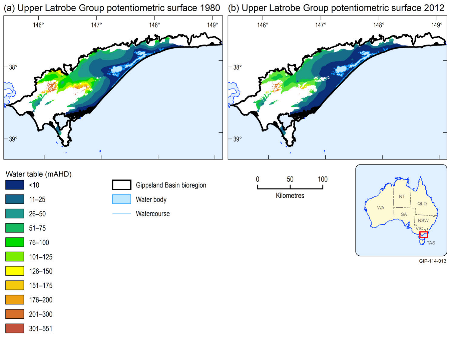
- Confined Latrobe Group sands below brown coal seams up to 135 m thick. The aquifers were artesian before development.
- The open-cut coal mines pump about 30 GL/yr to keep their floors stable. Offshore oil and gas production takes about 100 GL/yr more.
- Heads fell 120 to 130 m at the mines and about 1 m/yr across the region.
Land subsidence: 1 to 2.2 m near the mines and 0.3 to 0.5 m across the region, from compaction of coal and clay. The coast near the Gippsland Lakes fell 27 to 89 mm from 2004 to 2019.
Newer Volcanics, western Victoria
- More than 400 volcanic centres, Pliocene to Holocene, over about 19 000 km².
- Water moves through fractures, flow contacts and lava tubes; scoria cones store it.
K ranges from10^{-3} to10^{2} m/day. - Recharge is up to about 30 mm/yr at young volcanoes but 1 to 2 mm/yr through clay soils. Salinity rises from below 560 mg/L near vents to above 3000 mg/L on the plains.
- Use is about 23 GL/yr. Many basalt-plain wetlands depend on groundwater.
- The Atherton Tablelands basalt (Qld) is the same aquifer type in a wet climate: recharge 150 to 660 mm/yr, water less than 30 years old.
Northern Territory carbonates: the Tindall Limestone
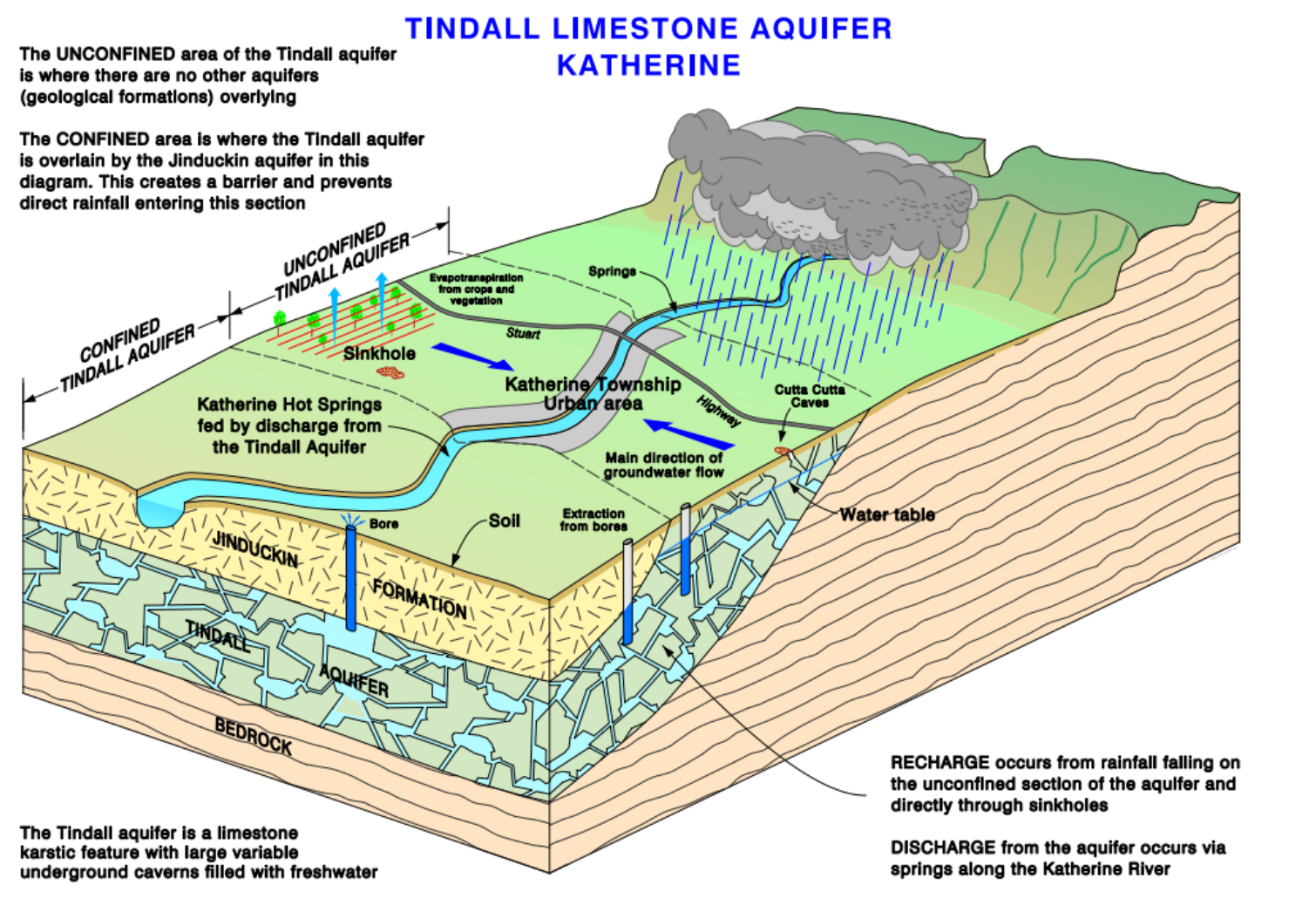
- Cambrian limestone and dolostone: the Tindall Limestone and Oolloo Dolostone of the Daly Basin.
- Karst:
T reaches 17 000 m²/day. Dye moved 570 to 1250 m/day from a sinkhole to springs. - About 70% of the monsoon recharge enters through sinkholes and macropores.
- Discharge keeps the Katherine and Daly rivers flowing through the dry season.
Licences are cut in dry years to protect river flow. Fire-fighting foam from RAAF Base Tindal put PFAS in the aquifer.
The Cambrian Limestone Aquifer
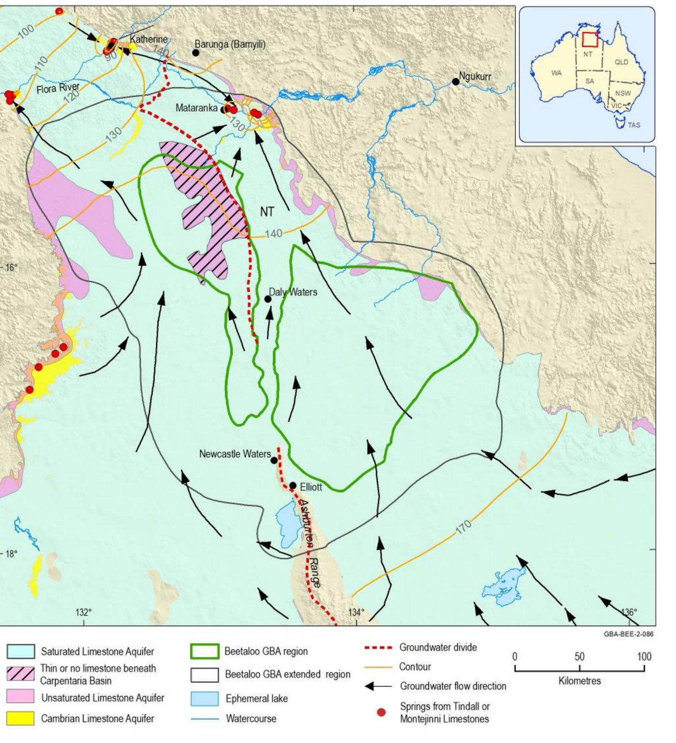
- One karst aquifer system across the Daly, Wiso and Georgina basins, about 570 000 km².
- Recharge follows the rainfall gradient: median about 82 mm/yr in the Daly Basin, 9 mm/yr in the Georgina Basin.
- Flow paths hundreds of kilometres long end at springs: Mataranka (25–33 °C), the Flora River and the Roper River.
- Water is mostly below 1000 mg/L TDS. Present use is small, but plans allow large increases.
The Beetaloo shale gas targets lie below this aquifer, separated by aquitards. How well those aquitards seal is not yet known.
Canning Basin
- The largest sedimentary basin in WA, about 430 000 km² onshore, and almost undeveloped.
- Broome Sandstone: unconfined, weakly consolidated. Coastal throughflow holds the seawater interface in place.
- Wallal Sandstone: confined below the Jarlemai Siltstone. On the coastal plain it is artesian, with heads 2 to 30 m above ground.
- Grant Group and Poole Sandstone (Fitzroy Valley): up to 2000 m thick and artesian. Water is up to 40 000 years old.
A resource in waiting
Fitzroy Valley use is about 5 GL/yr. A CSIRO assessment estimates that up to 170 GL/yr could be taken. The 120 GL/yr of this from the Grant–Poole aquifer is less than 5% of its recharge.
Groundwater discharge feeds the dry-season pools of the Fitzroy River and Mandora Marsh, which has the most inland mangroves in Australia.
Pilbara: Millstream and mine dewatering
Millstream aquifer
- Cainozoic dolomite and calcrete in the Fortescue valley: karst with cavities. Storage about 1.7 km³.
- Recharge comes mainly from floods. One cyclone flood in 1975 added about 49 GL.
- Springs feed 20 km of permanent river pools. A water-table fall of only 0.23 m reduced spring flow, so pumping now follows rules on minimum levels.
Iron-ore mines
- Mines below the water table must dewater. In 2012 the Pilbara abstracted about 400 GL/yr: 48% for mining and 40% as surplus mine water released to creeks.
- One mine next to the Fortescue Marsh is approved to pump up to 100 GL/yr and reinject most of it.
About 350 species of stygofauna, animals that live in groundwater, have been found in Pilbara aquifers.
Eucla Basin: the Nullarbor
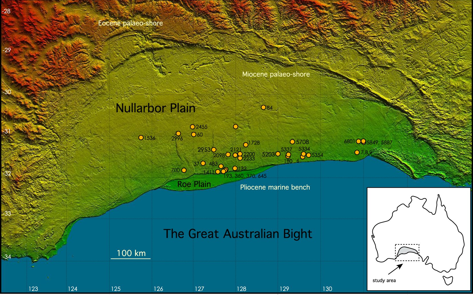
- Eocene to Miocene marine limestones (Wilson Bluff, Abrakurrie, Nullarbor): the largest area of exposed karst in the world.
- Rainfall is 150 to 250 mm/yr. Recharge happens only in rare large storms, through clay pans and blowholes.
- The water table is 30 to 120 m deep and almost flat.
- Mostly saline: about 6000 to 15 000 mg/L. Use is a few stock bores.
The caves formed in a wetter Pliocene climate. Most speleothems are 3 to 5 million years old.
Fractured rock: Yilgarn, Mount Lofty Ranges, eastern highlands
- Yilgarn (WA): deeply weathered Archean granite. Saprolite
K \approx 0.5 m/day; water up to more than 250 000 mg/L. Gold mines pump buried palaeochannel sands (K = 20–70 m/day) with water more than 100 000 years old. - Mount Lofty Ranges (SA): fractured metasediments.
K spans seven orders of magnitude. Clearing raised recharge from below 2 to about 60 mm/yr. - Eastern highlands and Tasmania: low-yield fold-belt rocks used for stock and domestic supply.
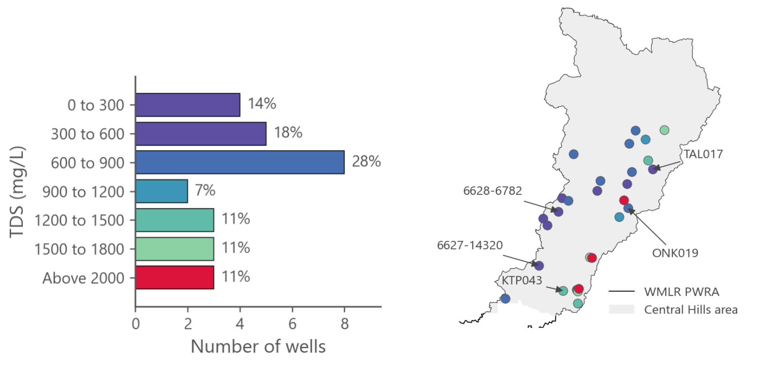
In 2000, 4.4 million ha of the WA Wheatbelt had a high potential to develop dryland salinity.
Queensland coastal alluvium
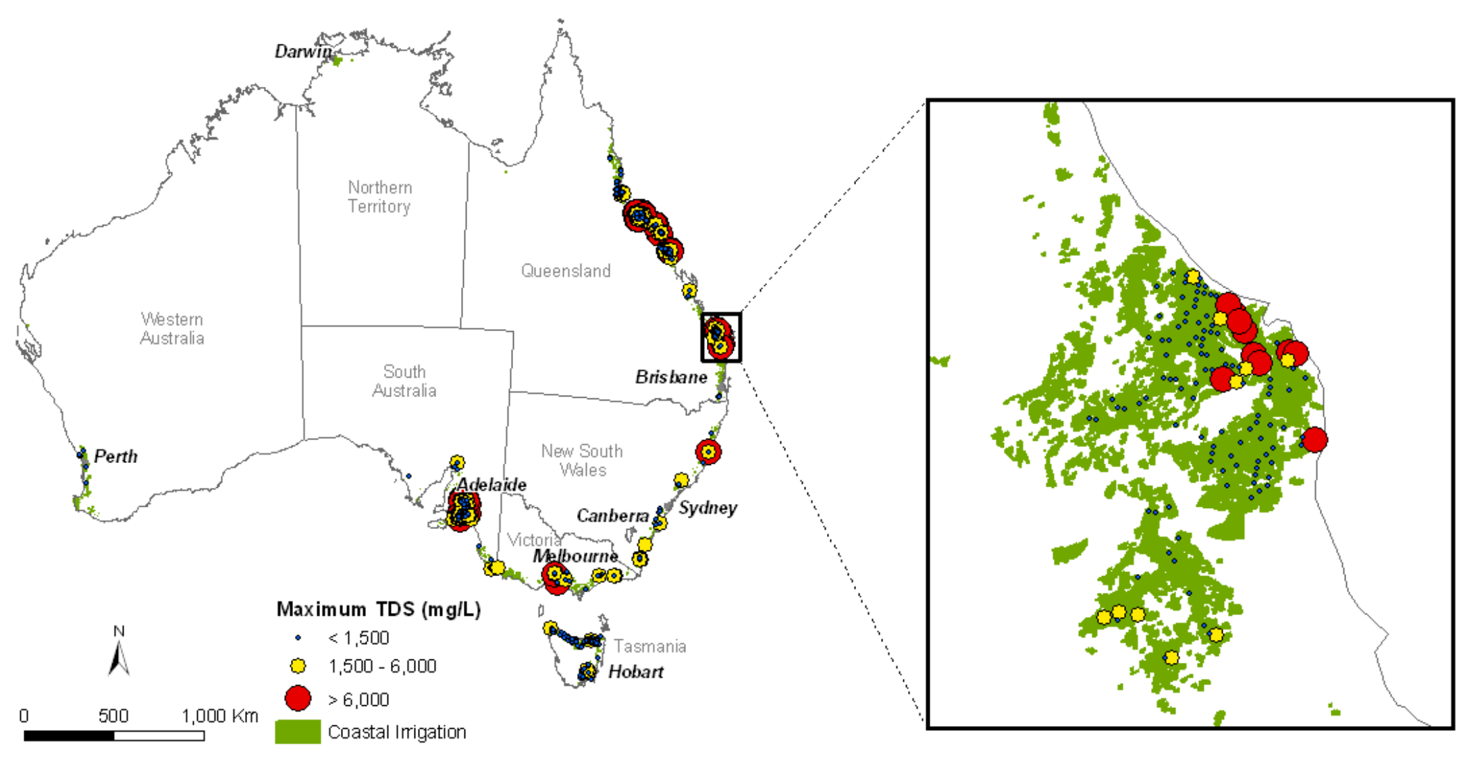
- Shallow, unconfined alluvium and delta sands, pumped for sugarcane.
- Burdekin delta: more than 100 m of sediment. River water has been put back underground since 1965, up to about 45 GL/yr.
- Pioneer Valley: pumping stops when the head in the aquifer above sea level falls below a trigger.
- Bundaberg: about 12 500 ha lost to seawater intrusion since the 1960s.
- Lockyer Valley (inland): use above the sustainable yield; no new bores since 2005.
Comparing Australian Aquifer Systems (1)
| System | Aquifer type | Recharge | Salinity (mg/L) | Main issue | |
|---|---|---|---|---|---|
| Great Artesian Basin | Confined sandstone | ~15 mm/yr | 500–1000 | Pressure loss | |
| Murray Basin | Layered sand, limestone | <0.1 to 40 mm/yr | 200–300 000 | Salinisation | |
| MDB alluvium | Sand and gravel | River leakage | <500–10 000 | Over-allocation | |
| Perth Basin | Sand over sandstone | ~120 mm/yr | mostly <1000 | Drying climate | |
| Otway Basin | Karst over sand | ~90 mm/yr | <500–10 000 | Plantations | |
| Gippsland Basin | Sand under coal | Basin margins | <500–3500 | Subsidence | |
| Newer Volcanics | Fractured basalt | 1–30 mm/yr | <560 to >3000 | Wetlands |
South and east. Typical ranges from Geoscience Australia, the Bureau of Meteorology and state reports.
Comparing Australian Aquifer Systems (2)
| System | Aquifer type | Recharge | Salinity (mg/L) | Main issue | |
|---|---|---|---|---|---|
| NT carbonates | Karst carbonate | 9–82 mm/yr | ~100–2000 | River baseflow | |
| Canning Basin | Sandstone, artesian | 0.3–85 mm/yr | <500–5000 | Future use | |
| Pilbara (Millstream) | Karst dolomite | Floods | 300–1500 | Springs, dewatering | |
| Eucla Basin | Karst limestone | not measured | Very low | 6000–15 000 | Saline |
| Fractured rock | Granite, metasediments | <2 to 60 mm/yr | <500 to >250 000 | Low yield | |
| Qld coastal alluvium | Sand | no data | Rain, river, MAR | <1500 to >6000 | Seawater intrusion |
North, west and fractured rock. Typical ranges from Geoscience Australia, the Bureau of Meteorology and state reports.
Summary
Key takeaways from this lecture:
Aquifer Classification:
- Aquifers are the fundamental unit of groundwater hydrology
- Three types: unconfined, confined, perched—each with distinct boundary conditions
- Confining beds range from impermeable (aquifuge) to leaky (aquitard), with complex real-world aquitardifers
Aquifer Properties:
- Transmissivity (
T = Kb ) quantifies ease of transmission; storativity (S ) quantifies storage release - Storage mechanisms: elastic (
S_s ) in confined, gravity drainage (S_y ) in unconfined aquifers - Relationship:
n = S_y + S_r connects porosity to drainable and retained water
Summary
Key takeaways from this lecture:
Real-World Aquifer Systems:
- Alluvial (Murray–Darling rivers): the most heavily pumped aquifers, recharged mostly by river leakage
- Sandstone (Great Artesian Basin): confined and artesian, with water more than one million years old
- Semiconsolidated (Murray, Gippsland): salinisation, seawater intrusion and land subsidence
- Carbonate and karst (NT, Mount Gambier, Nullarbor): very high transmissivity, springs that keep rivers flowing
- Fractured rock (Yilgarn, Mount Lofty Ranges): about 40% of the stored groundwater, but low yields
- Climate and land use change recharge: a drying climate in Perth, land clearing in the Mallee