- / -

EMSC3025/6025: Remote Sensing of Water Resources

Evaporation

EMSC3025/6025

Dr. Sia Ghelichkhan

Objectives

By the end of this lecture, you should be able to:

Explain the physical controls on evaporation.
Distinguish open-water, potential, and actual evaporation.
Explain how soil evaporation, transpiration, and interception combine to form evapotranspiration.
Compare field methods for measuring or inferring evaporation.
Apply the physical reasoning behind Penman and Penman—Monteith estimates.
Explain how thermal, optical, and microwave observations constrain satellite evaporation products.

Evaporation

Definition

Evaporation is the net transfer of water from a liquid surface to water vapour in the atmosphere.

Three conditions control the rate:

Energy must be available for vaporisation.
Liquid water must be available at, or transported to, the surface.
The atmosphere must remove the water vapour.

Climate determines how these controls combine. A humid winter can be energy-limited, while an arid summer is commonly water-limited.

flowchart TB
    L[Liquid water] -- vaporisation --> V[Water vapour]
    V -- condensation --> L
    E[Available energy] --> L
    M[Atmospheric mixing] --> V

Evaporation is a net molecular flux

Definitions used in hydrology

Three related fluxes

Open-water evaporation, E_o: evaporation from lakes, rivers, reservoirs, and oceans.
Potential evaporation, E_p: evaporation that the atmosphere could sustain from a specified surface with unlimited water.
Actual evaporation, E: evaporation that occurs under the existing water supply and surface conditions.

Potential evaporation is an atmospheric demand, not an observed loss. Actual evaporation can approach potential evaporation when water is abundant, but the relation depends on the reference surface, vegetation, and advection.

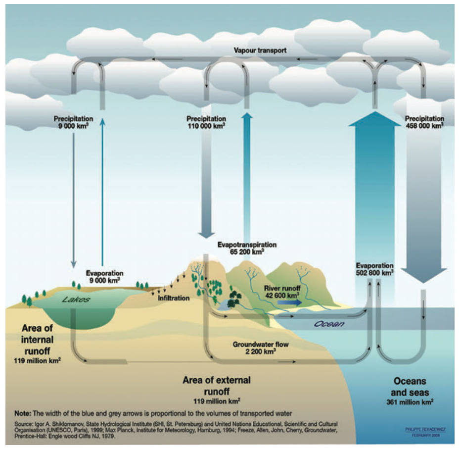Global Water Cycle Source: Davie and Quinn, Figure 1.7.

Components of terrestrial evaporation

flowchart TD
    E[Terrestrial evaporation] --> T[Transpiration]
    E --> B[Bare-soil evaporation]
    E --> I[Interception loss]
    E --> W[Open-water evaporation]

Components of evaporation above land

Evapotranspiration (ET) commonly denotes evaporation from soil and wet surfaces together with plant transpiration.

The relative contribution of each component changes with vegetation cover, rainfall history, soil moisture, and atmospheric demand. A satellite product that reports total ET does not necessarily observe, or even model, each component in the same way.

Transpiration, and a bit of fun with TSA

Transpiration: water through the soil—plant—atmosphere system

Water moves from soil to roots and through the xylem along a gradient in water potential.
Evaporation inside a leaf maintains tension in the xylem and water is lost through stomata.
Vapour pressure deficit increases atmospheric demand, while stomatal closure restricts the flux.
Stomatal opening also permits carbon dioxide uptake. Transpiration is therefore coupled to photosynthesis, but it is not caused by photosynthesis or respiration.

flowchart TB
    S[Soil<br/>−0.1 to −1 MPa] --> R[Roots]
    R --> X[Xylem]
    X --> L[Leaf<br/>−1 to −3 MPa]
    L --> A[Atmosphere<br/>much more negative]

Water follows a gradient in water potential

Corn sweat: a visible consequence of transpiration

Dense crops can add substantial water vapour to the atmospheric boundary layer during hot summer conditions.

The resulting humidity can increase heat stress, even though transpiration cools the crop surface. The example illustrates that transpiration redistributes both water and energy between the land and atmosphere.

The exact regional contribution depends on crop area, growth stage, soil water, wind, and boundary-layer mixing.

flowchart TB
    W[Soil water or irrigation] --> T[Crop transpiration]
    T --> H[Boundary-layer humidity]
    H --> S[Human heat stress]
    M[Wind and atmospheric mixing] -->|reduce accumulation| H

How crop transpiration affects local heat stress

Evaporation as a process

Dalton recognised that evaporation depends on wind and the difference in vapour pressure between a wet surface and the surrounding air:

E = C (e_s(T_s) - e_a)

e_s(T_s) is the saturated vapour pressure at the surface temperature T_s.
e_a is the actual vapour pressure of the air.
C represents turbulent transport and therefore depends on wind, roughness, and atmospheric stability.

This expression describes the aerodynamic control. It does not separately account for the energy required to vaporise water.

Two controls

Atmospheric demand

e_s(T_s)-e_a

Turbulent transport

wind + surface roughness + stability

The radiation balance

Net radiation is the balance of incoming and outgoing short-wave and long-wave radiation:

R_n = (K_\downarrow-K_\uparrow) + (L_\downarrow-L_\uparrow)

K_\downarrow and K_\uparrow: incoming and reflected short-wave radiation.
L_\downarrow and L_\uparrow: atmospheric and surface long-wave radiation.

Surface albedo controls reflected short-wave radiation. Surface temperature and emissivity control outgoing long-wave radiation. Satellites can constrain all three properties.

flowchart TB
    SUN[Sun] -->|incoming short-wave K↓| S[Land surface]
    S -->|reflected short-wave K↑| SKY[Atmosphere and space]
    ATM[Atmosphere] -->|incoming long-wave L↓| S
    S -->|outgoing long-wave L↑| SKY

Radiative fluxes at the surface

How the surface uses available energy

After allowing for heat storage and horizontal advection, the surface energy balance is approximately

R_n - G = H + \lambda E

G: ground or water-body heat flux.
H: sensible heat flux to the atmosphere.
\lambda E: latent heat flux used for evaporation.

A wet surface directs a larger fraction of available energy into \lambda E and commonly remains cooler. A dry surface directs more energy into H and commonly becomes warmer.

flowchart TD
    R[Net radiation R_n] --> G[Ground heat G]
    R --> H[Sensible heat H]
    R --> LE[Latent heat lambda E]
    W[Water availability] --> LE
    LE -. surface cooling .-> T[Land-surface temperature]

Partition of available energy

Water supply

Over oceans and large lakes, water supply is effectively unlimited. The main controls are available energy, vapour pressure gradients, and atmospheric mixing.

Over land, evaporation is often restricted because water must reach the evaporating surface. Soil texture, hydraulic conductivity, surface crusting, rooting depth, and antecedent rainfall all affect this transport.

After a wetting event, bare-soil evaporation commonly passes through two stages:

An energy-limited stage while the surface remains wet.
A transport-limited stage after the surface dries and water must move upward through the soil.

Roots provide a separate pathway from deeper soil to the leaves, but stomatal regulation can restrict that flux.

The receiving atmosphere

At a specified air temperature, the vapour pressure deficit is

\mathrm{VPD}=e_s(T_a)-e_a

and relative humidity is

\mathrm{RH}=100\,e_a/e_s(T_a).

VPD measures atmospheric demand at the air temperature. The vapour-pressure gradient above a wet surface also depends on the surface temperature, so VPD and Dalton’s surface-to-air difference are related but not identical.

Wind and turbulence replace moist air near the surface with drier air and sustain evaporation.

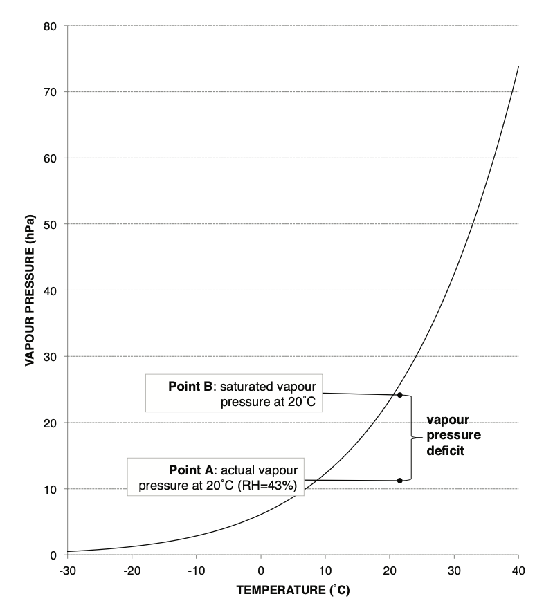
Vapour pressure deficit at 20 degrees Celsius.

Source: Davie and Quinn, Figure 3.2.

Evaporation depends on its environment

The same atmosphere does not produce the same evaporation from a lake, bare soil, pasture, and forest.

Open-water and soil evaporation

Open-water evaporation

Water supply is not normally limiting.
Surface temperature, salinity, depth, and heat storage matter.
Wind, VPD, fetch, and atmospheric stability control removal of vapour.
A pan is not a small lake because its sides, heat storage, and edge effects alter the flux.

Soil evaporation

The surface can change rapidly from wet to dry.
Soil water transport limits the flux after the surface dries.
Residue, vegetation cover, albedo, and roughness modify both energy and transport.
The same meteorological conditions can therefore produce much less evaporation than over open water.

Transpiration and total evaporation

Transpiration depends on:

available soil water and rooting depth,
hydraulic transport through the plant,
VPD and turbulent mixing,
stomatal response to environmental stress.

Total terrestrial evaporation combines transpiration, bare-soil evaporation, interception loss, and any open-water evaporation within the area.

flowchart LR
  S[Soil water<br/>and roots] --> C[Plant hydraulic<br/>supply]
  C --> ST[Stomatal<br/>control]
  A[VPD, radiation,<br/>wind] --> ST
  ST --> T[Transpiration]

Transpiration needs both water supply and atmospheric demand

Climate and vegetation redistribute evaporative loss

Estimated water balances for two Pinus radiata forests.
Component	Puruki, central North Island	Balmoral, central South Island
Annual rainfall	1,405 mm	870 mm
Interception loss	370 mm (26%)	220 mm (25%)
Transpiration	705 mm (50%)	255 mm (29%)
Soil evaporation	95 mm (7%)	210 mm (24%)
Runoff + percolation	235 mm (17%)	185 mm (21%)

The annual interception fraction is similar, but transpiration and soil evaporation differ strongly. Climate and vegetation determine not only total evaporation, but also its partition into components.

Source: Kelliher and Jackson (2001), as reproduced by Davie and Quinn.

How do we observe evaporation?

No single instrument measures every relevant scale

A rain gauge catches a depth of water. There is no equivalent gauge that catches the water vapour leaving a catchment.

Evaporation is instead inferred from:

turbulent fluxes above a surface,
changes in water storage,
the surface energy balance,
meteorological and remotely sensed variables.

Each method has a spatial support:

a lysimeter represents a small plot,
an eddy-covariance tower represents a changing upwind footprint,
a satellite pixel represents a mixed area,
a catchment balance integrates the full drainage area.

Agreement requires more than matching units. The spatial and temporal supports must also be compatible.

Eddy covariance

Eddy covariance estimates the turbulent water-vapour flux from the covariance between fluctuations in vertical wind and water-vapour density:

E \propto \overline{w' q'}

A three-dimensional sonic anemometer and a fast gas analyser commonly sample at 10—20 Hz.

The method is direct in the micrometeorological sense, but it still requires corrections, quality control, and an estimate of the source footprint. Calm conditions, non-stationarity, heterogeneous terrain, and incomplete energy closure remain important limitations.

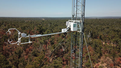OzFlux eddy-covariance instruments Source: OzFlux, Collie monitoring site.

Flux-gradient and Bowen-ratio methods

Aerodynamic profile

Vertical gradients in wind, temperature, and humidity are related to turbulent transport using similarity theory.

The method requires well-resolved profiles, surface roughness, and atmospheric-stability corrections. It is most reliable over horizontally uniform terrain with an adequate fetch.

Bowen ratio

The ratio of sensible to latent heat is inferred from temperature and vapour-pressure gradients:

\beta = \frac{H}{\lambda E} = \gamma\frac{\Delta T}{\Delta e}.

Combined with R_n-G=H+\lambda E, this gives the latent heat flux. Small or changing humidity gradients can make the estimate unstable.

Water-balance inference

For storage change defined as \Delta S=S_{end}-S_{start},

\Delta S = P-Q-E

and therefore

E=P-Q-\Delta S.

A water balance infers evaporation as the residual. It does not measure evaporation independently, and errors in every other term accumulate in E.

flowchart TD
  P[Precipitation P] --> S[Storage S]
  S --> Q[Runoff or drainage Q]
  S --> E[Evaporation E]
  D[Observed storage change] --> E

Water-balance estimate

Evaporation pans

A closed pan has no runoff or drainage, so

E=P-\Delta S.

A Class A pan provides a long and relatively simple record of open-water evaporation. It does not measure actual evaporation from a catchment.

The small water body has strong edge effects, absorbs heat through its sides, and stores energy differently from a lake. Empirical pan coefficients are therefore required even when estimating lake evaporation.

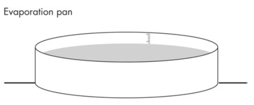Evaporation pan Source: Davie and Quinn, Figure 3.3.

Lysimeters

A lysimeter contains soil and vegetation that approximate the surrounding surface. With measured drainage Q,

E=P-Q-\Delta S.

A weighing lysimeter measures storage change directly and can resolve actual evapotranspiration over a plot. Its accuracy does not remove the scale problem: soil disturbance, vegetation mismatch, edge effects, and a small sampled area can limit representativeness.

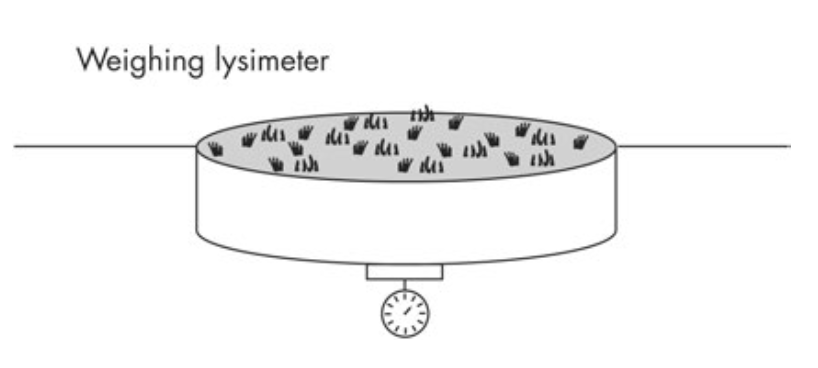Weighing lysimeter Source: Davie and Quinn, Figure 3.4.

Estimating evaporation from surrogate variables

Field instruments cannot provide continuous evaporation over every catchment. Estimation methods therefore use variables that control the flux, including temperature, radiation, wind, humidity, soil moisture, and vegetation.

Increasing model complexity does not make the result a direct measurement. It changes which assumptions and observations determine the estimate.

flowchart LR
  T[Temperature] --> TH[Thornthwaite]
  R[Radiation + VPD + wind] --> P[Penman]
  C[Canopy + aerodynamic resistance] --> PM[Penman--Monteith]
  S[Satellite surface state] --> RS[Observation-constrained models]

Progression of evaporation estimates

Thornthwaite

Thornthwaite is an empirical monthly estimate of potential evaporation based primarily on mean air temperature.

i = \left( \frac{T}{5} \right)^{1.514}, \qquad I = \sum_{j=1}^{12} i_ja = 6.75 \times 10^{-7} I^3 - 7.71 \times 10^{-5} I^2 + 0.01792 I + 0.49239

E_p = 16 b \left( \frac{10T}{I} \right)^a

The factor b corrects for day length and month length. The method is economical when data are sparse, but temperature is only a proxy for radiation and atmospheric demand.

It commonly underestimates potential evaporation in hot, arid environments where VPD and radiation are not represented explicitly.

Penman: energy and aerodynamic demand

Penman combines an energy term with an aerodynamic term for a wet surface:

E_o = \frac{\Delta Q^* + \gamma E_a}{\Delta + \gamma},

where the wind function can be written in the empirical form

E_a = 2.6\,\delta_e\left(1+\frac{u}{1.862}\right).

Here Q^* must be expressed in evaporation-equivalent units, \delta_e is the vapour-pressure deficit, u is wind speed, \Delta is the slope of the saturated vapour-pressure curve, and \gamma is the psychrometric constant.

The estimate depends on the quality of the radiation, temperature, humidity, and wind data. Heat storage and advection can be important for water bodies and wet surfaces.

Priestley—Taylor

Priestley and Taylor simplified the combination approach for extensive wet surfaces where regional advection is limited:

\lambda E_p = \alpha\frac{\Delta}{\Delta+\gamma}(R_n-G).

The coefficient \alpha empirically enhances equilibrium evaporation. Priestley and Taylor obtained \alpha\approx1.26 for extensive saturated surfaces, but it is not universal.

The method requires fewer meteorological inputs than Penman, which made it attractive for early satellite applications.

Its assumptions become weak over heterogeneous or water-limited land. Modern products therefore add stress factors, use additional observations, or retain the aerodynamic term.

Penman—Monteith: from a wet surface to a canopy

Monteith added surface resistance to represent stomatal and canopy control:

E = \frac{\Delta (R_n-G) + \rho_a c_p\,\mathrm{VPD}/r_a}{\lambda\left[\Delta+\gamma\left(1+r_s/r_a\right)\right]}.

r_a: aerodynamic resistance to turbulent transfer.
r_s: bulk surface or canopy resistance.

As r_s approaches zero, the surface approaches the wet-surface Penman case under consistent aerodynamic assumptions.

A large r_s restricts transpiration, but neither resistance is fixed. Both depend on surface structure and environmental conditions.

Reference evapotranspiration and crop coefficients

FAO reference evapotranspiration, ET_o, is defined for a hypothetical well-watered grass surface that is 0.12 m high, has surface resistance 70 s/m, and has albedo 0.23.

Crop evapotranspiration is commonly estimated as

ET_{crop}=K_c ET_o.

The crop coefficient varies with growth stage, canopy height and cover, albedo, soil evaporation, climate, and management.

A value above or below one cannot be attributed only to roughness or stomatal control. The coefficient integrates several differences between the crop and reference surface.

Source: Allen et al. (1998).

From potential to actual evaporation

Soil moisture provides a first-order constraint on the ratio E/E_p. The relation is nonlinear and depends on soil hydraulic properties, rooting depth, vegetation, and the definition of E_p.

A single stress curve can be useful in a water-balance model, but it does not represent all plant responses or atmospheric feedbacks.

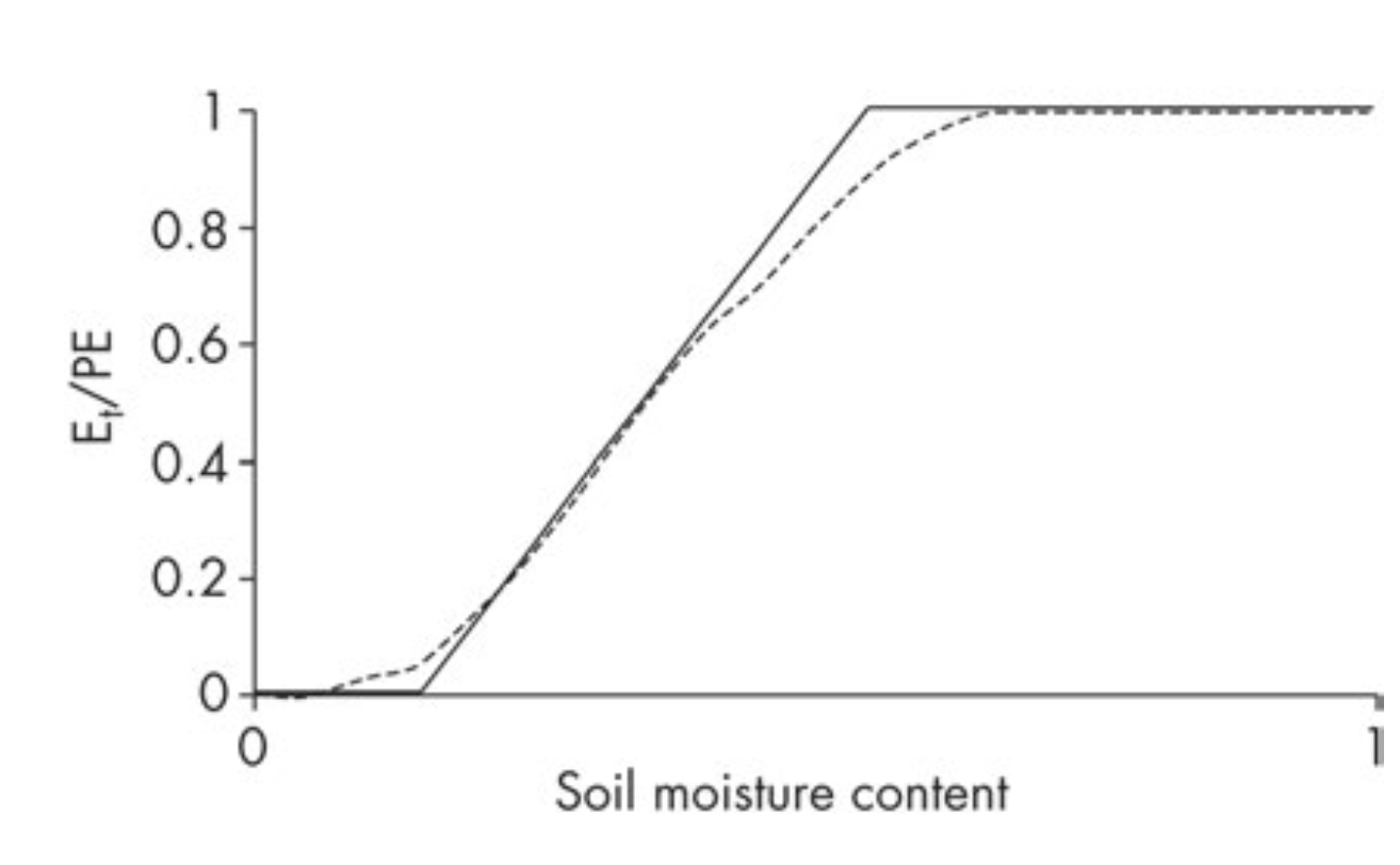Soil moisture stress Source: Davie and Quinn, Figure 3.10.

Vegetation responds to both supply and demand

The Pinus radiata record separates three controls:

In early summer, adequate soil moisture permits transpiration to increase with atmospheric demand.
Transpiration then plateaus while VPD increases, which is consistent with stomatal regulation.
Later, transpiration decreases as soil moisture becomes limiting, even when VPD remains appreciable.

A vegetation index alone cannot distinguish these controls.

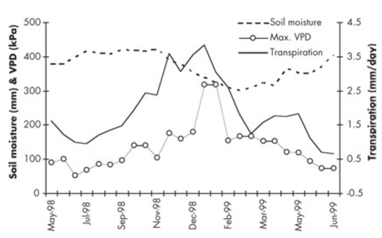Transpiration, soil moisture, and VPD Source: Davie and Quinn, Figure 3.11; data courtesy of Rick Jackson.

Scaling up: observation-constrained evaporation from space

What does a satellite measure?

A satellite records electromagnetic radiance, brightness temperature, or radar backscatter. Evaporation is not one of these quantities.

The observation must first be converted into a surface property and then combined with a model.

flowchart TD
  O[Measured radiance or backscatter] --> R[Retrieved surface property]
  R --> M[Evaporation model]
  F[Meteorological forcing] --> M
  M --> E[Estimated evaporation]
  G[Ground observations] --> V[Validation or calibration]
  V --> M

The observation chain

Thermal infrared: evaporation cools the surface

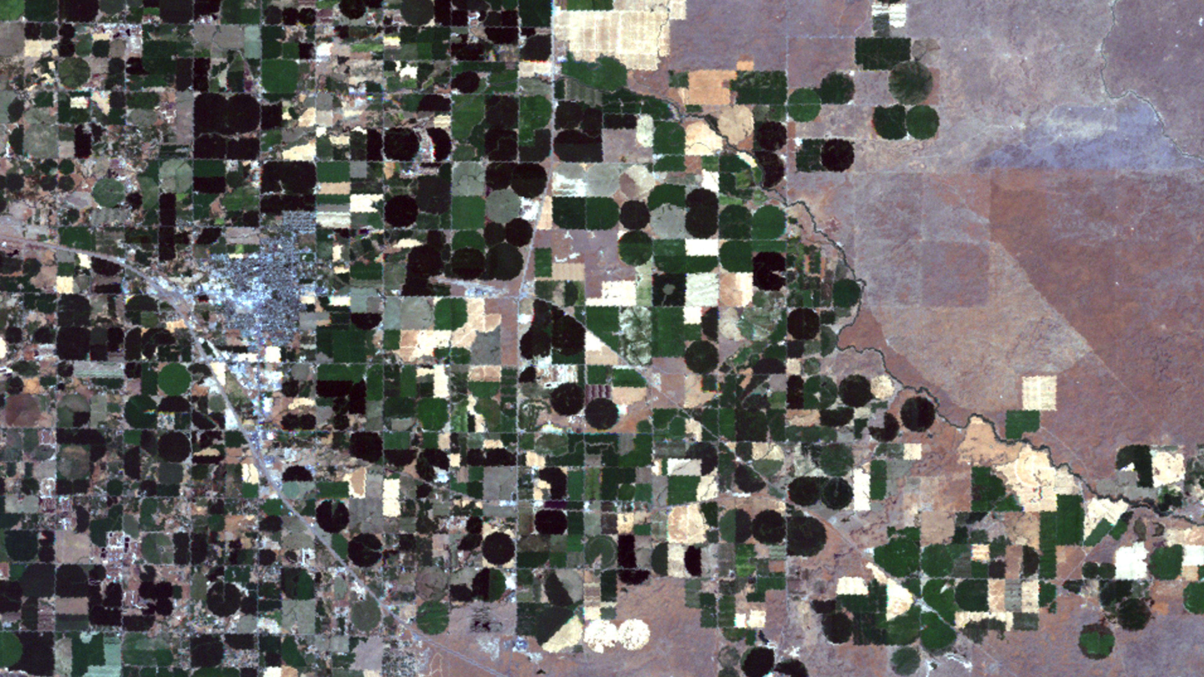Visible Landsat image Visible reflectance

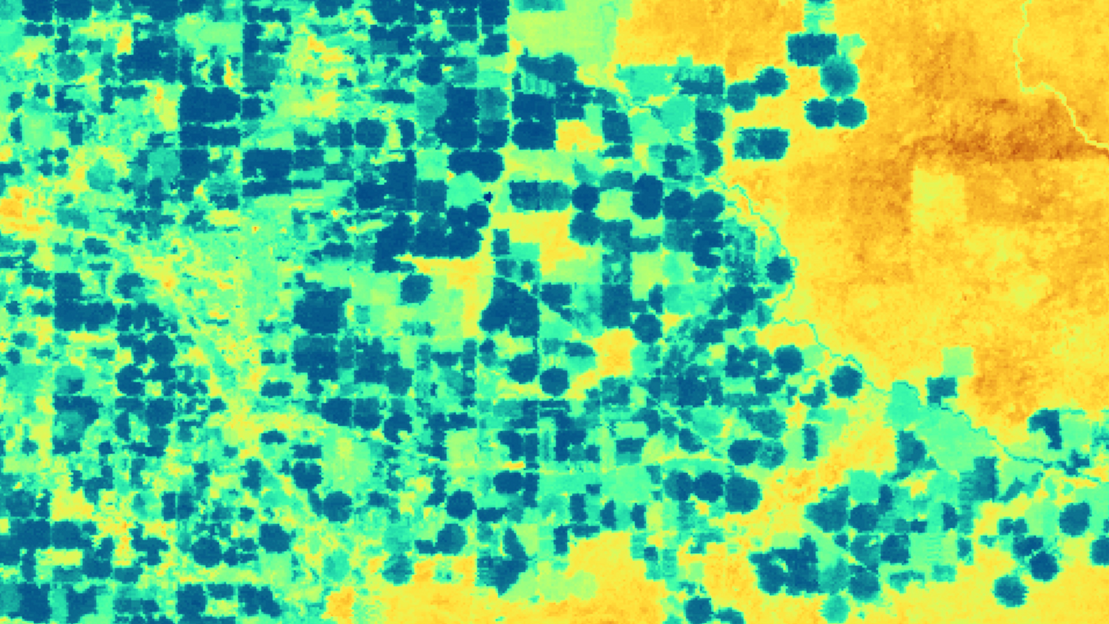Thermal Landsat image Land-surface temperature

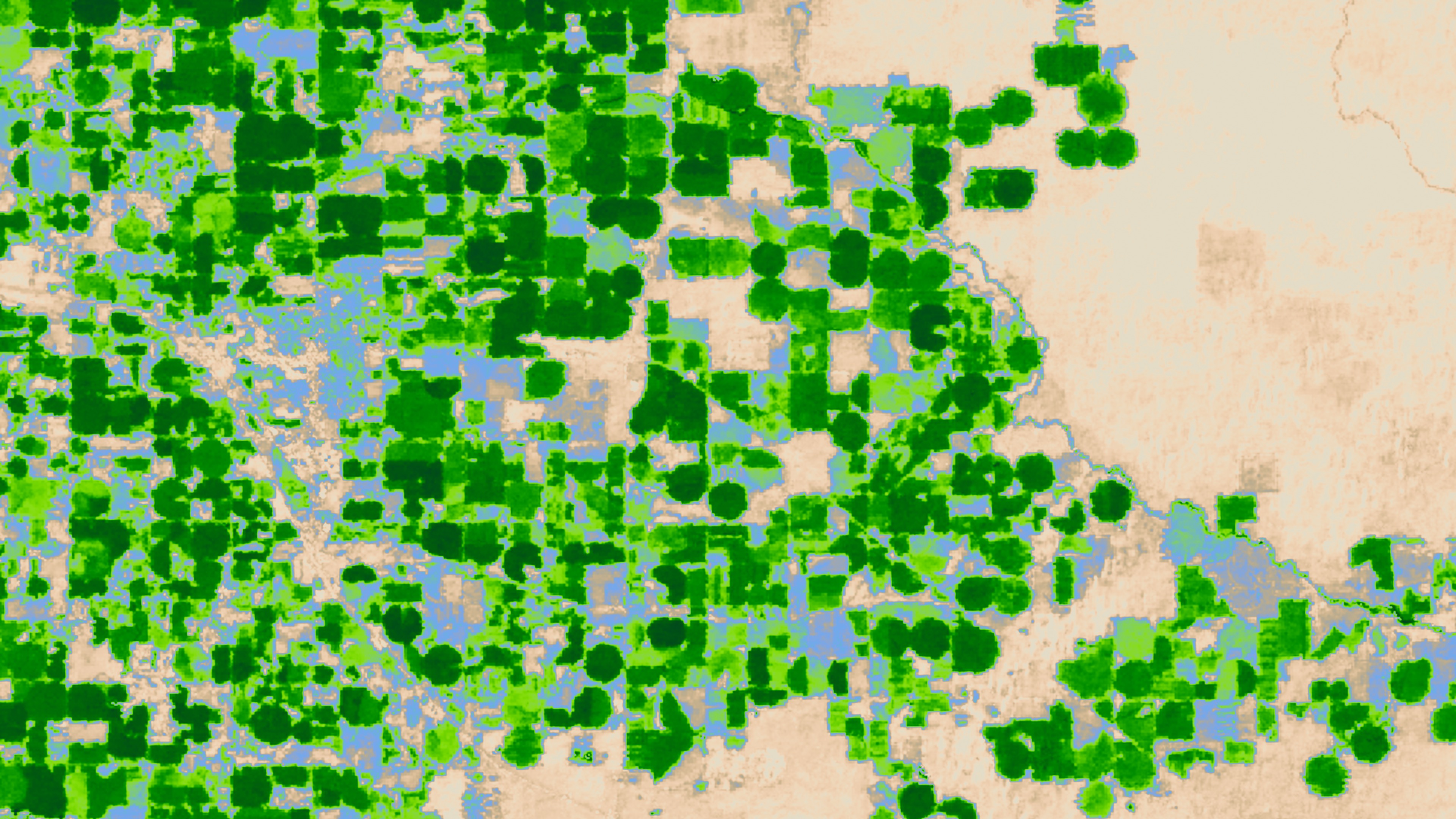METRIC evaporation map Modelled ET

Evaporating fields are cooler because latent heat consumes available energy. Thermal radiance constrains surface temperature, not ET directly. Clouds, emissivity, atmospheric correction, and temporal upscaling remain important limitations. Source: NASA/GSFC Scientific Visualization Studio (2009).

Optical observations: vegetation and surface properties

Optical sensors measure reflected solar radiation. Combinations of spectral bands retrieve properties that influence evaporation:

red and near-infrared reflectance constrain vegetation cover and greenness through NDVI or EVI,
short-wave infrared reflectance responds to vegetation and surface water content,
broadband albedo constrains absorbed radiation.

These variables do not uniquely determine evaporation.

A green canopy can close its stomata during high VPD. Vegetation indices can saturate over dense canopies, clouds remove observations, and a pixel can mix soil, vegetation, and water.

CMRSET uses EVI and the Global Vegetation Moisture Index to scale potential evaporation.

Microwave observations: water supply and stress

Passive microwave radiometers measure brightness temperature. Active radar measures backscatter. Retrieval algorithms use their sensitivity to dielectric properties to estimate near-surface soil moisture.

Microwave vegetation optical depth provides information about vegetation water content and biomass. These observations help constrain whether potential evaporation can be sustained.

The observation chain is indirect:

Microwave signal
Surface soil moisture or VOD retrieval
Root-zone model or stress factor
Evaporation estimate

Passive microwave pixels are coarse, the sensing depth is shallow, and vegetation and surface roughness affect the retrieval.

This is the same active/passive observation principle used by the ESA CCI soil-moisture product in Assignment II.

Two families of satellite evaporation models

Surface energy balance

\lambda E = R_n-G-H

Thermal surface temperature, albedo, vegetation cover, and meteorological data constrain the energy terms. Examples include SEBAL, METRIC, and ALEXI/ECOSTRESS.

The surface temperature is especially important for estimating sensible heat H.

Potential evaporation with stress

E = S\,E_p, \qquad 0\leq S\leq1

Penman or Priestley—Taylor provides atmospheric demand. Soil moisture, VOD, vegetation indices, and land-cover information constrain the stress factor.

GLEAM and CMRSET use variants of this approach. MOD16 uses Penman—Monteith with satellite vegetation properties and meteorological forcing.

GLEAM: the Davie and Quinn case study

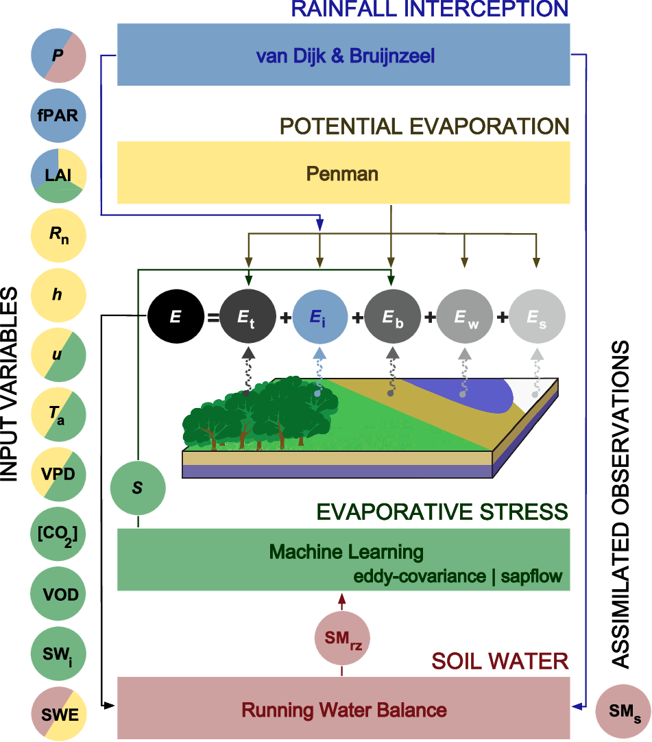
GLEAM4 schematic — Input observations, model modules, and output fluxes in GLEAM4.

Davie and Quinn describe GLEAM v3, which used Priestley—Taylor at 0.25 degree resolution and assimilated microwave soil-moisture observations.

GLEAM4 now uses Penman at 0.1 degree resolution. It combines satellite and reanalysis observations of radiation, temperature, vegetation, soil moisture, wind, and VPD. Separate modules estimate transpiration, bare-soil evaporation, interception, open-water evaporation, sublimation, and condensation.

The transition from v3 to v4 shows that an evaporation product is a changing model system, not a fixed satellite measurement.

Source: Miralles et al. (2025), Scientific Data, CC BY 4.0.

CMRSET: actual evaporation across Australia

The original CSIRO MODIS Reflectance-based Scaling Evapotranspiration model used MODIS EVI and GVMI to scale Priestley—Taylor potential evaporation.

The current TERN v2.2 product blends Landsat, Sentinel-2, MODIS, and VIIRS observations to provide monthly actual evaporation at 30 m resolution without persistent cloud gaps.

The model was calibrated against OzFlux eddy-covariance sites and evaluated against water balances for unregulated catchments.

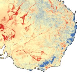CMRSET Australia Source: ANU Centre for Water and Landscape Dynamics; Guerschman et al. (2009).

CMRSET and AWRA-L answer different questions

CMRSET

Scales potential evaporation with optical vegetation and moisture indices.
Resolves fields and wetlands at 30 m and monthly intervals.
Is well suited to spatial water-use and irrigation studies.
Depends on cloud-gap filling, meteorological forcing, and empirical calibration.

AWRA-L

Simulates the daily landscape water balance on a coarser national grid.
Represents soil stores, runoff, drainage, and evaporation together.
Provides the Australian Water Outlook evaporation used in the tutorial.
Is not fully independent of CMRSET because CMRSET information contributed to AWRA-L calibration.

How do we validate a satellite evaporation product?

Validation must compare compatible spatial and temporal supports:

a lysimeter represents a plot,
a flux tower represents an upwind footprint that changes with the wind,
a satellite pixel can contain several land covers,
a catchment balance integrates storage and lateral flow.

Agreement at one scale does not guarantee that the component fluxes or short-term variability are correct.

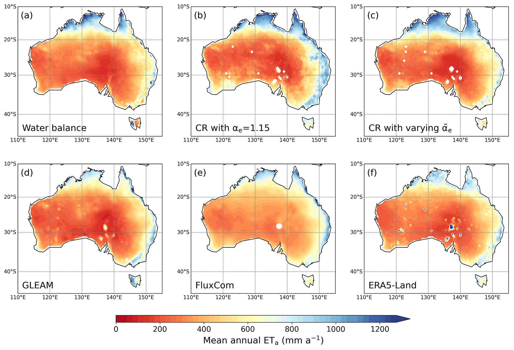Australian evaporation product comparison Source: Kim et al. (2022), Hydrology and Earth System Sciences, Figure 7, CC BY 4.0.

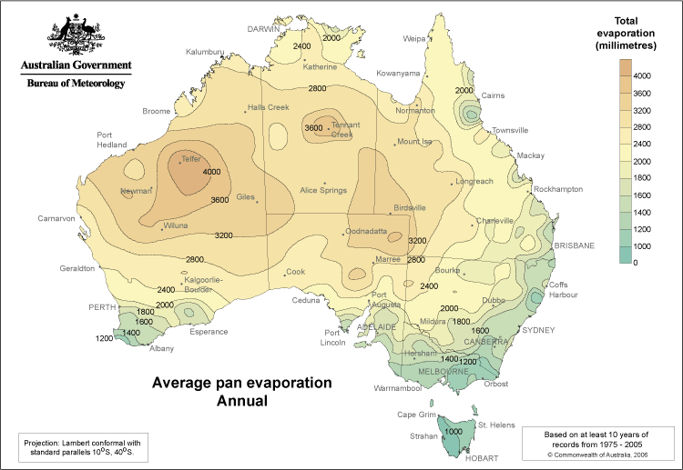
The Australian contrast: demand is not actual loss

Australian pan evaporation Source: Bureau of Meteorology, CC BY 4.0.

Class A pan evaporation exceeds 3,000 mm/year across much of inland Australia. This records strong atmospheric demand over an unlimited water supply.

Actual terrestrial evaporation is much lower across the arid interior because soil and vegetation cannot sustain that demand. It is higher in wetter northern and coastal regions despite lower pan evaporation.

The contrast is the continental expression of the lecture’s central distinction:

\text{atmospheric demand} \neq \text{actual water loss}.

Summary

Evaporation requires available energy, available water, and atmospheric transport.
The surface energy balance partitions net radiation between ground, sensible, and latent heat fluxes.
Eddy covariance estimates turbulent flux, while pans, lysimeters, and catchment balances infer evaporation at different scales.
Penman and Penman—Monteith combine energy supply with atmospheric and surface resistance.
Satellites observe radiance or backscatter, not evaporation.
Thermal, optical, and microwave observations constrain models of surface energy and water stress.
Every evaporation product must be interpreted through its model, spatial support, forcing data, and validation evidence.