- / -
EMSC3025/6025: Remote Sensing of Water Resources

Groundwater — Principles
EMSC3025/6025
Dr. Sia Ghelichkhan
Objectives
By the end of this module, you will be able to:
- Porosity and conductivity: explain why porosity tells you how much water a rock holds, but not how fast the rock releases it
- Hydraulic head: explain why head controls the direction of flow and pressure does not, and calculate head from a field measurement
- Darcy’s law: calculate specific discharge and pore velocity, and state when the law fails
- Origin of Darcy’s law: show why conductivity increases with the square of the grain size, and use this to explain the empirical formulas for
K - Layered ground: calculate the equivalent horizontal and vertical conductivity, and explain how layering alone can make horizontal conductivity a million times larger than vertical conductivity
- Field data: interpret piezometer nests, potentiometric maps and water-level hydrographs
- GRACE: explain how satellite gravity measures total water storage, and how the groundwater part is separated from it
Two separate questions
This lecture answers two questions about a volume of soil or rock.
1. How much water does it hold?
Porosity answers this. It depends on the amount of void space.
2. How fast can the water flow out?
Hydraulic conductivity answers this. It depends on how the voids connect.
A common mistake is to assume that the answer to one question gives the answer to the other. It does not. Clay has one of the highest porosities of the materials in this lecture, and one of the lowest conductivities.
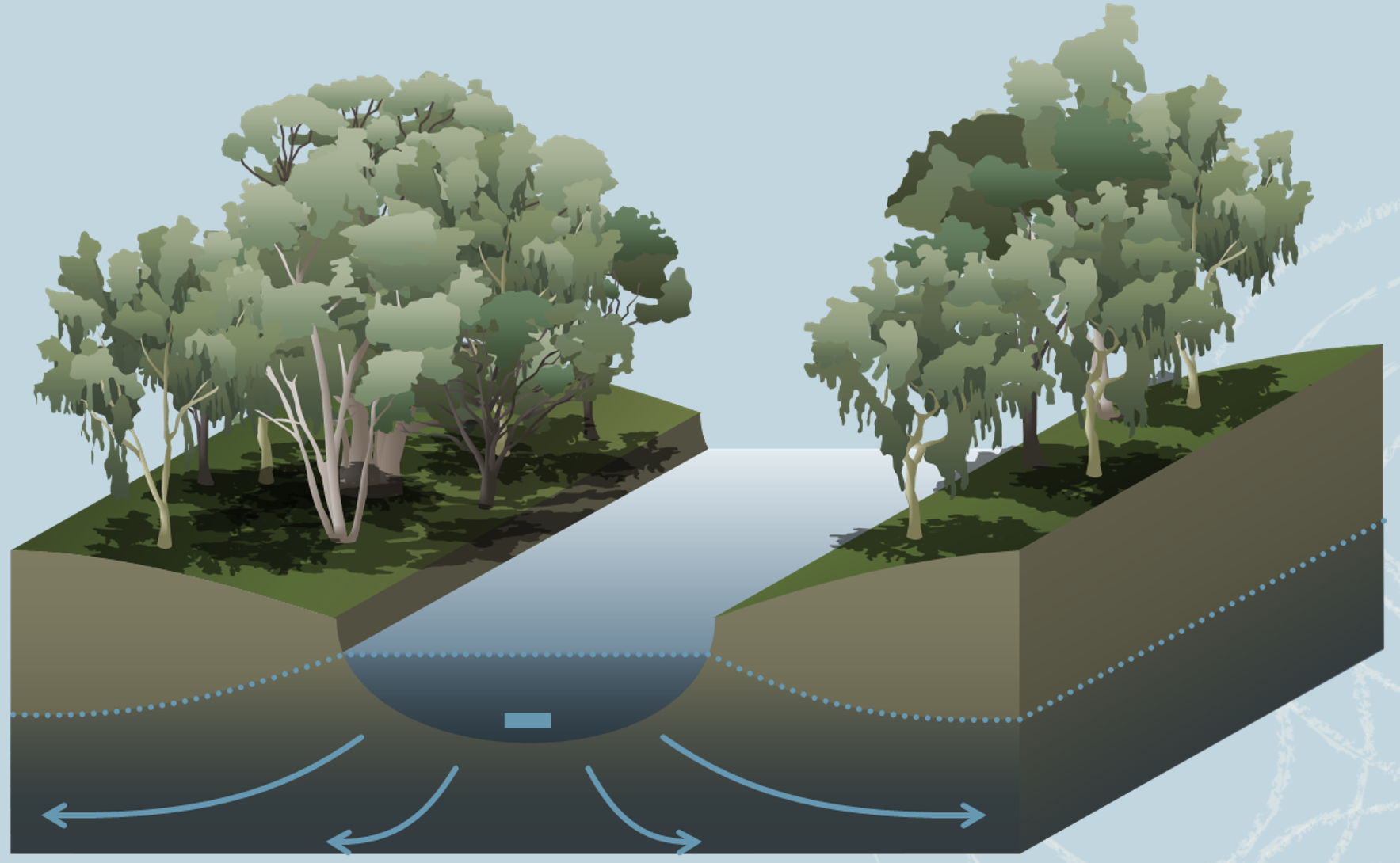
Porosity: how much water the ground holds
Porosity of a Soil or Rock
- Porosity is the fraction of a volume of rock or soil that is void space.
- Total porosity
n_T is defined as:n_T = \frac{V_v}{V_T} = \frac{V_T - V_s}{V_T} whereV_v is the volume of voids,V_s the volume of solids andV_T the total volume. - Since
V_v < V_T , porosity is always a fraction below 1. It is often quoted as a percentage. - In the laboratory it is easier to weigh than to measure void volume, so the same quantity is obtained from densities:
n_T = 1 - \frac{\rho_b}{\rho_s} with\rho_b the bulk density of the dry sample and\rho_s the particle density of the solids. - For most silicate minerals
\rho_s \approx 2650 kg/m³, so a dry bulk density of 1600 kg/m³ givesn_T = 0.40 .
What sets porosity: packing
For grains of one size, porosity is set by how they are stacked.
Take identical spheres. The loosest stable stacking is cubic, each sphere sitting directly on the one below:
n_T = 1 - \frac{\pi}{6} = 0.476 The tightest is rhombohedral, each sphere resting in the hollow between three others:
n_T = 1 - \frac{\pi}{3\sqrt{2}} = 0.260
Both numbers are independent of the size of the spheres. Void volume and total volume both increase with the cube of the radius, so their ratio stays the same. A box of marbles and a box of beach balls have the same porosity.
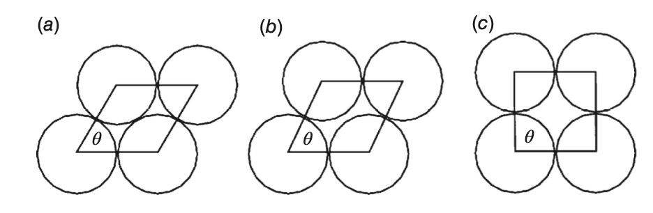
Compaction pushes the grains of a real sediment from the loose arrangement towards the tight one. This lowers the porosity without changing the grain size.
What sets porosity: sorting and shape
- Sorting is the spread of grain sizes in a sample.
- Well sorted (one size): porosity is close to the sphere-packing values on the previous slide.
- Poorly sorted (mixed sizes): small grains fill the voids between large ones, and porosity is lower.
- Glacial till, a mix of sand, silt and clay, is the usual example. Its mean porosity is 23.5%, the lowest of the unconsolidated materials in the porosity table later in this section.
- Grain shape can raise or lower porosity. Angular and flat grains can prop each other up and keep voids open that spheres would fill. They can also fit together tightly and close voids that spheres would leave open. Shape alone does not tell you which effect wins.
- Clays reach 40 to 55%. Surface charges hold their flat particles edge to face, which gives an open structure with a lot of void space. The small size of the particles is not the reason.
A common misconception
In the table of measured values, finer materials tend to have higher porosity. This is a pattern in the data. It does not mean that small grains cause high porosity. In a well-sorted material, grain size has no effect on porosity. Clay is porous because of the shape and charge of its particles.
Grain size does control conductivity: later in this lecture we show that
Primary and Secondary Porosity
- Primary porosity: the voids that formed with the rock.
- Pores between grains in a sediment or sandstone
- Vesicles, lava tubes and cooling fractures in basalt
- Secondary porosity: voids created afterwards.
- Joints and faults in igneous, metamorphic and consolidated sedimentary rock
- Solution-enlarged openings in carbonates and other soluble rock
- The two types behave differently. Primary porosity is spread through the whole rock. Secondary porosity is concentrated in fractures and openings, which may or may not connect to each other.
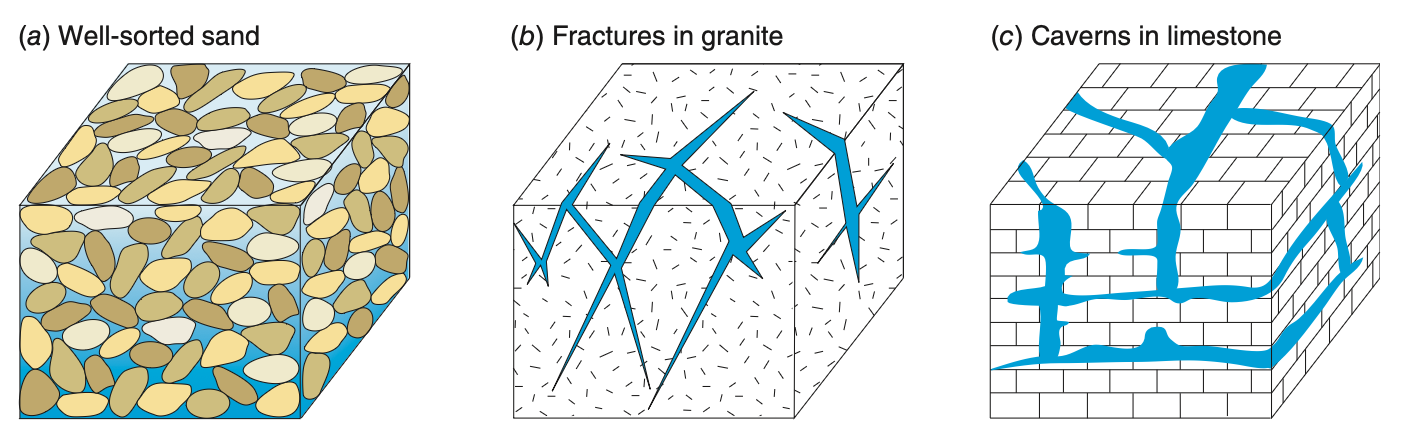
The name of a rock, for example “limestone”, tells you little about its porosity. Its history of fracturing and dissolution tells you much more.
Porosity in natural materials
| Material | Min | Mean | Max | SD |
|---|---|---|---|---|
| Unconsolidated deposits | ||||
| Sand | 28.1 | 38.9 | 44.4 | 4.9 |
| Dune | c | 42.1 | c | 8.3 |
| Silt | 31.5 | 45.2 | 50.8 | 5.6 |
| Clay | 40.1 | 46.1 | 55 | 4.5 |
| Glacial till | 14.3 | 23.5 | 34 | c |
| Peat | c | 92 | c | c |
Values in per cent. “c” means there were too few measurements to give a value. Field values for sand and gravel are usually lower, 25 to 35%, because the laboratory samples in this table were loosely packed.
| Material | Min | Mean | Max | SD |
|---|---|---|---|---|
| Sedimentary rocks | ||||
| Sandstone | 4 | 20.4 | 28.6 | 8.6 |
| Limestone | 0.44 | 8.67 | 34.7 | 8.6 |
| Dolostone | 0.4 | 7.46 | 26 | c |
| Shale | 0.75 | 10.8 | 27.2 | 8.3 |
| Igneous rocks | ||||
| Granite | <0.001 | 0.01 | ||
| Basalt | <0.01 | 0.1 |
Sandstone has lower porosity than sand because mineral cement fills part of the pore space. Burial and chemical change after deposition (diagenesis) reduce porosity further with age and depth. Unfractured igneous rock has almost no porosity, so in granite nearly all the water is in fractures like those in the figure two slides back.
Effective porosity
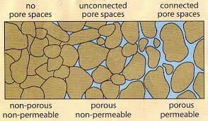
Water cannot flow through every void. Effective porosity
n_e is the fraction of the volume made up of voids that connect to each other, so that water can flow through the sample.In a clean sand or gravel all the pores connect, and
n_e \approx n_T .In a fractured rock they do not. The pores of a shale hold water but connect poorly, so the water that flows, flows in the fractures. The fracture porosity
n_f is then the effective porosity.Below the weathered zone near the surface, fractures are typically tens to hundreds of micrometres wide. Fractures 100 µm wide and one metre apart give
n_f = \frac{10^{-4}\,\mathrm{m}}{1\,\mathrm{m}} = 10^{-4} Typical fracture porosities are
10^{-4} to10^{-3} . The total porosity of the same shale is about 0.10, which is up to a thousand times larger.
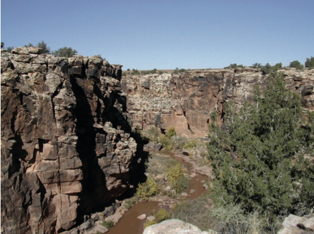
Schwartz & Zhang p. 45 gives
Dual porosity
A fractured rock has two porosities, and each one has a different role.
| Matrix | Fractures | |
|---|---|---|
| Porosity | 0.05 – 0.15 | |
| Holds the water | yes | no |
| Carries the flow | no | yes |
- The matrix (the rock between the fractures) holds almost all of the water. The fractures carry almost all of the flow.
- A contaminant in the fractures slowly diffuses into the matrix. After clean water has replaced it in the fractures, it diffuses back out for decades. This is why contaminated fractured rock is so hard to clean up. We return to this later in the course.
- Karst works in the same way, except that dissolution has widened the fractures into conduits.
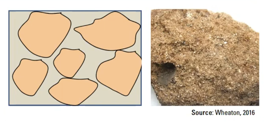
Same porosity, very different yield
Two wells drilled to the same depth, in two materials with the same porosity of 0.30.
| Gravel | Silt | |
|---|---|---|
| Porosity | 0.30 | 0.30 |
| Water stored per m³ | 300 L | 300 L |
| Hydraulic conductivity | ||
| Yield to a well | supplies a town | fills a bucket |
Both materials hold the same amount of water. Only the gravel releases it to a well at a useful rate.
The extreme case: clay
Clay has a mean porosity of 46%, among the highest in the porosity table. It also has the lowest hydraulic conductivity of the sediments in the conductivity figure later in this lecture. Clay is nearly half water by volume, but a well in clay yields almost nothing.
- Porosity sets storage.
- Conductivity sets transmission.
- An aquifer needs both. A unit with high porosity and low conductivity is a confining bed. Next week’s lecture covers aquifers and confining beds.
Occurrence: where the water sits
Occurrence of Groundwater
- Near the surface the pores hold both water and air. This is the unsaturated zone. Its water content rises when water infiltrates and falls when plants take it up or it evaporates. Plants get their water from this zone, and the soil moisture lecture covers it.
- Deeper, the pores hold only water: the saturated zone, and the water in it is groundwater.
- The water table separates the two. It is the surface on which water pressure equals atmospheric pressure.
- Just above the water table, surface tension holds up a saturated layer at below-atmospheric pressure. This is the capillary fringe. By the definition above it is not groundwater. It is millimetres thick in gravel and metres thick in clay.
- Water that passes below the roots and reaches the water table is recharge.
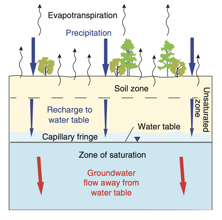
Flow of Groundwater
- Recharge arrives at the water table and then moves down and sideways towards a discharge point: a river, a spring, a wetland, the sea.
- One quantity drives both the downward and the sideways motion: the gradient in hydraulic head. The next section defines head and shows why its gradient differs from the pressure gradient.
- Surface runoff and groundwater discharge reach the same river, but they take very different times to get there.
- Groundwater discharge is the baseflow from the runoff lecture. A river keeps flowing after months without rain because water that fell in earlier years is still reaching it.
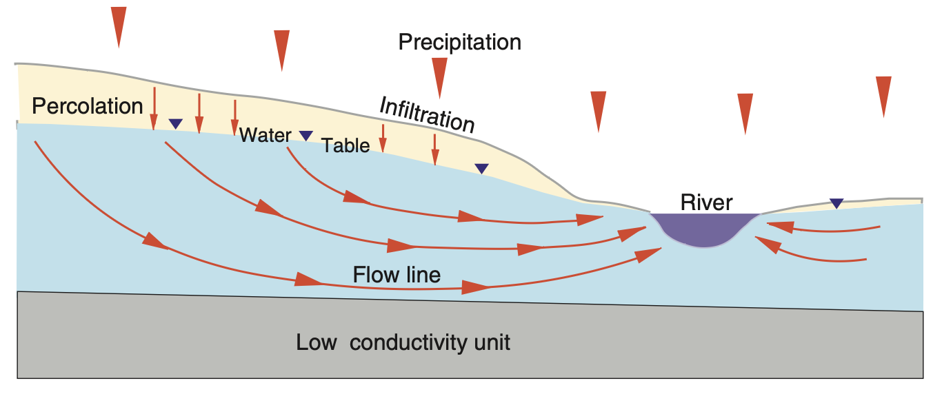
Surface runoff reaches the stream in hours. Groundwater takes years.
How long does it take?
Residence time is the length of the flow path divided by the speed of the water. The formula for the speed comes from Darcy’s law, later in this lecture:
| System | |||
|---|---|---|---|
| Hillslope to creek, sand | 300 m | 0.15 m/day | 5 years |
| Small basin, sand and gravel | 20 km | 0.5 m/day | 100 years |
| Great Artesian Basin | 1000 km | 1 m/year |
- The water in a bore in western Queensland fell as rain on the Great Dividing Range before the last glacial period.
- This is the same residence time as in the water cycle lecture, but calculated for one flow path instead of a whole reservoir.
Why this matters for management
A store with a residence time of
The groundwater management lecture returns to this, and Assignment III uses the same calculation.
Groundwater flow in the lab
Hydraulic head: what sets the direction of flow
Pressure does not set the direction of flow
Take a column of water standing still in a tube. Pressure at depth
- The pressure at the bottom is larger than the pressure at the top. If water always flowed from high to low pressure, it would flow upward.
- But nothing moves. The column is in equilibrium.
- The same is true below a water table. Pressure increases with depth everywhere, even where the water is not moving at all.
Pressure alone cannot tell you the direction of flow. The quantity that can is hydraulic head.
Pressure changes from the top to the bottom of the column, but head stays the same. Where head is constant, there is no flow, however the pressure varies.
Hydraulic head
The energy of a unit weight of water at a point has three parts. This is the Bernoulli equation, written in units of length:
z : elevation head, the height of the point above the datum, usually sea level. This is the gravitational part.P/\rho_w g : pressure head, the height of the water column the pressure would support.v^2/2g : velocity head, the kinetic part.
Groundwater moves at about 1 m/day, which is
compared with head differences of metres. We therefore ignore the velocity head:
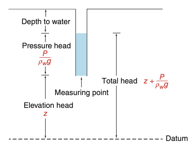
Going down the still column, the pressure head increases by exactly as much as the elevation head
Measuring head in the field
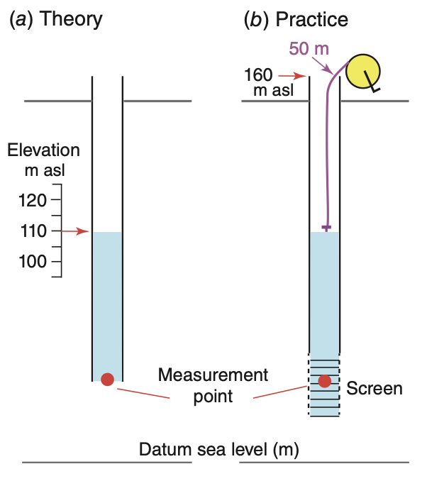
The water level in a standpipe that is open at the bottom gives the head at the open end.
In principle (a): read the elevation of the water level against a scale. In the figure it is 110 m above sea level.
In practice (b): the pipe has no scale on it, so head is calculated from two measurements.
- Survey or high-precision GPS gives the elevation of the top of casing,
EL_{TOC} = 160 m. - A weighted electric tape gives the depth to water,
DTW = 50 m.
h = EL_{TOC} - DTW = 160 - 50 = 110\ \mathrm{m} - Survey or high-precision GPS gives the elevation of the top of casing,
This is the head at the measurement point, the middle of the screen at the bottom of the pipe. It is not the head at the water table.
The screen is a slotted section of casing that lets water in. Its open area lets the water level in the pipe follow changes in the ground, which matters most in low-conductivity ground.
One site, two heads
Two pipes at one site, screened at different depths. The shallow one reads 84 m. The deep one reads 73 m.
- Both readings are correct. This site has no single “groundwater level”.
- Head is 11 m lower at depth, so the hydraulic gradient points downward. Water flows from the shallow unit into the deep aquifer.
- Head belongs to a point. A head measurement has no meaning until you state the depth of the screen and the unit it is in.
- This is why piezometers are installed in nests: three short screens at three depths at one location, to measure how head changes with depth.
- A well with a long screen gives an average head over the full length of the screen. At a site like this, it cannot show the vertical gradient.
Three types of well
- Water wells: wide casing, long screen. Many thousands already exist, so they are the only practical source of data for regional studies. They work well in a single aquifer where flow is horizontal. There, lines of equal head (equipotentials) are vertical, so the depth of the screen does not change the reading.
- Piezometers: narrow casing, short screen, sealed above with bentonite clay. They measure head at a point. They are used at contaminated sites, for dewatering, and in nests to measure vertical gradients.
- Water table observation wells: a long screen that covers the full range of water table depths, so the water table is always somewhere in the screen.
The observation well differs from the other two. Its measurement point is not the middle of the screen. It is the water table, which moves up and down through the year. Pressure head at the water table is zero, so head there equals the elevation of the water table.
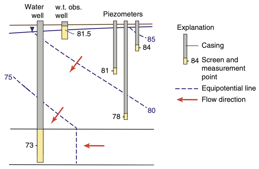
In the figure the nest reads 84, 81 and 78 m from shallow to deep. Head decreases with depth, so flow in the shallow unit is downward.
Darcy’s law
Darcy’s experiment
Henry Darcy, a civil engineer, built the water supply of Dijon in the 1850s. He needed to know how large to make the sand filters.
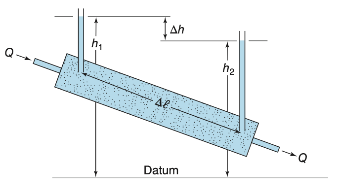
His apparatus was a cylinder of cross-section area
A , packed with sand. Water flowed through it at a measured rateQ . Two manometers a distance\Delta l apart measured the headsh_1 andh_2 .He changed the flow rate, the head difference, the length of the column and the type of sand, and found one relationship:
\frac{Q}{A} = -K \frac{dh}{dl} K , the hydraulic conductivity, includes all the properties of the sand. Darcy measuredK . He did not derive it. A derivation came about a century later, and we do it later in this section.Darcy’s law is an empirical law, like Ohm’s law, and it has the same form: a flux proportional to the gradient of a potential.
Darcy’s law, and its sign
q = Q/A is the specific discharge, also called the Darcy velocity. It is the volume of water per unit time through a unit area of the whole column face, in m/day.dh/dl is the change in head per metre along the directionl . The minus sign makes water flow in the direction in which head decreases.- You can also define the gradient as a positive head loss over a positive distance:
i = \frac{h_1 - h_2}{\Delta l} \quad (h_1 > h_2) Thenq = Ki , and the flow is from point 1 towards point 2. Both forms are in use. Choose one and use it consistently.
The textbook’s equation 3.5 uses
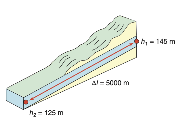
The gradient has no units: here the head falls by four millimetres for each metre of distance.
Darcy velocity and pore velocity
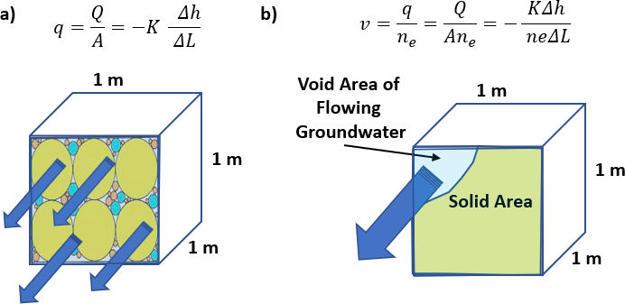
q is the discharge divided by the area of the whole column face, including the solid grains. No water actually travels at speedq .Water flows only through the connected voids, which make up a fraction
n_e of the face. The average linear velocity, or pore velocity, is thereforev = \frac{q}{n_e} = -\frac{K}{n_e}\frac{dh}{dl} Because
n_e < 1 ,v is always larger thanq .Use
v to calculate travel times, for example how long a contaminant takes to reach a bore.
Worked example: sand and fractured shale
Use
(a) Granular sand,
(b) Fractured shale, same
What the result means
Both rocks have the same conductivity, the same gradient and the same discharge
- A spill above the fractured shale reaches a bore 1 km away in three months. Above the sand it takes 24 years.
- This is why effective porosity is worth measuring. The misprinted value
n_f = 0.05 would give 0.7 m/day, a wrong answer that makes the site look safer than it is.
Note: the textbook prints 0.152 m/day as the answer to (a). Its own numbers give 0.115 m/day.
Where Darcy’s law comes from
Darcy measured
For laminar flow in a tube of diameter
Write the pressure in terms of head,
The specific discharge is
Three results from the derivation
q is proportional to the gradient, as Darcy observed. This is true only while the flow in the tubes is laminar.K has two factors:c\,d^2 depends on the rock, and\rho_w g/\mu depends on the fluid. The rock part is the intrinsic permeability, later in this lecture.K increases with the square of the pore diameter, and pore diameter increases with grain diameter. Every empirical formula forK in the next section is a form ofK \propto d^2 .
Grains ten times larger give a conductivity one hundred times larger. This explains most of the range of
Where Darcy’s law fails
Too fast: turbulence. The derivation assumed laminar flow. To test this, calculate a Reynolds number from the grain diameter:
and the law holds for
| Setting | |||
|---|---|---|---|
| Sand aquifer | 1 m/day | 1 mm | 0.01 |
| Coarse gravel | 100 m/day | 10 mm | 12 |
| Karst conduit, near a pumped well | much larger | much larger |
At higher
Too slow: a threshold. In clays with very low permeability, charged mineral surfaces hold the nearby water tightly. The water may not move at all until the gradient is larger than a minimum value (Bolt and Groenevelt, 1969).
Both failures happen only at the extremes. In nearly every aquifer, Darcy’s law is accurate enough, and the theory lecture builds on it.
This course covers two cases where the law fails in practice: karst conduits, in the aquifers lecture, and the area directly around a pumping well, in the well hydraulics lecture.
Conductivity, permeability, and how to estimate them
Hydraulic conductivity: twelve orders of magnitude
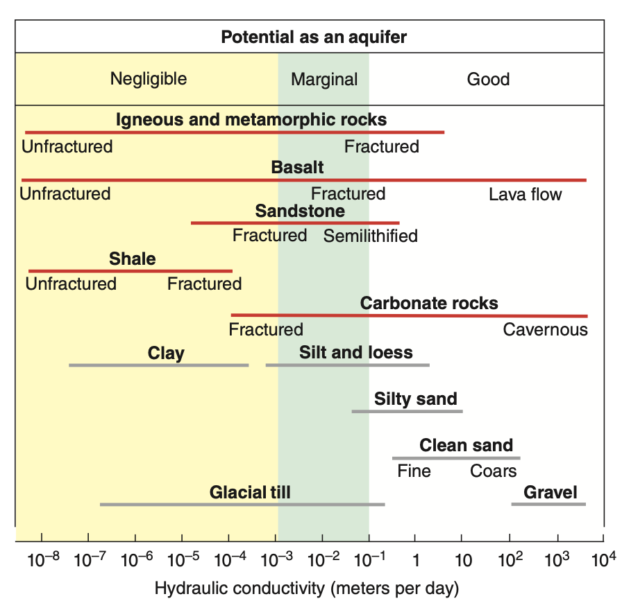
K has units of length over time. Values range from10^{-8} m/day in unfractured igneous rock to10^{4} m/day in limestone with caverns.- Few other properties in the earth sciences vary over twelve orders of magnitude. The porosity of most sediments and sedimentary rocks, for comparison, stays between about 1% and 50%.
What this means for a site investigation. An error of a factor of two in the gradient gives an error of a factor of two in the flow. An error in the type of material can give an error of a factor of
- In the figure, fractured rock of each type has a conductivity 10 to 1000 times higher than the same rock without fractures.
Intrinsic permeability
The derivation split
k is the intrinsic permeability, with units of area:\mathrm{m^2} , or\mathrm{cm^2} , or darcy, where1\ \mathrm{darcy} = 9.87\times10^{-13}\ \mathrm{m^2} .- It is an area because it is the
c\,d^2 from the derivation, which is proportional to the cross-section of a pore. - At 20 °C and 1 atm, with
\rho_w = 998.2 kg/m³ and\mu = 1.002\times10^{-3} kg/(m s):K = 9.77\times10^{6}\ \mathrm{m^{-1}s^{-1}} \cdot k k = 1.023\times10^{-7}\ \mathrm{m\,s} \cdot K
Why use k instead of K?
Temperature changes
| 5 °C | 1.00 | |
| 25 °C | 1.71 |
The same rock has a conductivity 1.7 times higher at 25 °C than at 5 °C, although the rock itself has not changed.
Estimating K from grain size
The derivation gave
| Source | Equation |
|---|---|
| Hazen (1911) | |
| Harleman (1963) | |
| Kozeny–Carman |
d_{10} is the effective grain size: the sieve opening that lets through 10% of the sample by weight. 90% of the sample is coarser.- Only Kozeny–Carman includes porosity, through
n^3/(1-n)^2 , and it shows the fluid factor\rho_w g/\mu explicitly. It is the bundle-of-tubes derivation with a more careful treatment of the pore shape.
Why the tenth percentile and not the mean?
Because the smallest grains (the fines) control the flow. In a sand with 10% clay, the clay particles fill the narrow openings between the sand grains. These openings control the resistance to flow, so the clay lowers
The same idea returns later in this lecture, in the vertical conductivity of layered ground. There too, the least conductive material controls the result.
Example from the tutorial:
Measuring K in the laboratory: constant head
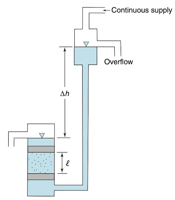
Used for coarse material,
Hold the head difference
h fixed across a core of lengthL and cross-section areaA .When the flow is steady, measure the outflow rate
Q by collecting water for a known time.Rearrange Darcy’s law to get
K = \frac{QL}{Ah} The overflow at the top keeps the supply head constant. Without it, the head falls as the reservoir drains, and the flow is no longer steady.
This is the same set-up as Darcy’s experiment.
Measuring K in the laboratory: falling head
Used for fine material: fine sands through to clays.
There is no constant supply. Water in a standpipe of cross-section area
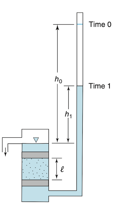
a drains through the core, and the head falls fromh_0 toh_1 in timet_1 - t_0 :K = 2.3\,\frac{aL}{A(t_1-t_0)}\log_{10}\!\left(\frac{h_0}{h_1}\right) The choice of test is practical. In a clay, the flow
Q in a constant-head test is too small to measure, but a falling water level is easy to measure. The standpipe is narrow (a is much smaller thanA ), so a small volume of flow gives a large drop in level.
Both tests measure a core a few centimetres across, which the coring has disturbed. The next section asks whether this value describes the whole aquifer.
Real ground: heterogeneous and anisotropic
Heterogeneity and anisotropy
Each red outline shows how far water travels from a point in one unit of time. A circle means that
- Homogeneous or heterogeneous asks whether
K changes from place to place. - Isotropic or anisotropic asks whether
K changes with direction at one place. - The two properties are independent, and all four combinations occur. Real ground is usually heterogeneous and anisotropic, as in the bottom right box.
The main point of this section: heterogeneity at a small scale becomes anisotropy at a larger scale. A stack of layers, each of them isotropic, behaves as one anisotropic material when you look at the stack as a whole.
K varies within a single unit
Thirty-two measurements of
| value (m/s) | |
|---|---|
| smallest | |
| largest | |
| arithmetic mean | |
| geometric mean | |
| harmonic mean |
- The values span four orders of magnitude, in one unit that a geological map shows as a single colour.
- The three means differ by a factor of 46. If you give “the” conductivity of a unit, you must say which mean you used.
- A histogram of
K is strongly skewed, but a histogram of\log K is close to a normal distribution.K is log-normally distributed. In this sample the mean of\log K is-7.0 and its standard deviation is0.76 . - This is why hydrogeologists use geometric means and plot conductivity on logarithmic axes.
Which mean is the right one?
It depends on the direction of flow relative to the layers. The next two slides show why:
- flow along the layers: arithmetic mean
- flow across the layers: harmonic mean
- any other case lies between the two (Matheron, 1967). If
K varies in the same way in every direction, the geometric mean is the usual estimate.
Layers in parallel: the arithmetic mean
Flow along the bedding. Each layer has the same head drop over the same distance, so each has the same gradient
a thickness-weighted arithmetic mean.
The most conductive layer controls
Each layer carries
Layers in series: the harmonic mean
Flow across the bedding. Now the same
a harmonic mean.
Now the least conductive layer controls
Electrical resistors behave in the same way. In parallel, the path with the lowest resistance carries most of the current. In series, the largest resistance controls the total.
The two grey layers make up a fifth of the thickness but cause nearly all of the head loss. A piezometer nest through this stack would show almost constant head in the sandy layers, and a steep drop in head across the grey ones.
Worked example: layering makes anisotropy
A 300 m sequence of interbedded sandstone and shale, 75% sandstone. Both rocks are isotropic.
- Sandstone:
K = 1\times10^{-5} m/s, 225 m in total - Shale:
K = 1.92\times10^{-12} m/s, 75 m in total
What the two answers mean
- Neither rock is anisotropic. The factor of a million comes only from the layering.
- So you cannot say whether a rock is anisotropic without saying at what scale you look at it.
- This is why regional groundwater models with 500 m cells use
K_h/K_v ratios of10^2 to10^4 : each cell contains many layers.
Anisotropy at two scales
Measured on a core
| Material | Horizontal | Vertical | Ratio |
|---|---|---|---|
| Anhydrite | 10 | ||
| Chalk | 2 | ||
| Limestone, dolomite | 2 | ||
| Sandstone | 2 | ||
| Shale | 10 | ||
| Salt | 1 |
- A core samples one bed. At that scale, anisotropy comes from flat grains that lined up when they were deposited, and the ratio is about 2 to 10.
- The much larger ratios in regional models come from layering, as calculated on the previous slide.
The word “anisotropy” covers two different causes at two different scales. When you give a ratio, say which one you mean.
- In both cases, water flows easily along a sedimentary sequence and with great difficulty across it. This is what makes confined aquifers possible.
Darcy’s law when direction matters
In an anisotropic material,
Each component of the flow depends on all three components of the gradient:
- The tensor is symmetric,
K_{xy} = K_{yx} , so six numbers describe it. - If you choose the coordinate axes along the principal directions of anisotropy, the off-diagonal terms are zero. For layered rock, these directions are along and across the bedding:
q_x = -K_{xx}\frac{\partial h}{\partial x},\quad q_y = -K_{yy}\frac{\partial h}{\partial y},\quad q_z = -K_{zz}\frac{\partial h}{\partial z}
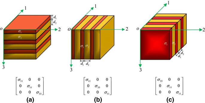
In anisotropic ground, flow lines do not cross equipotential lines at right angles. Right angles are correct only in isotropic ground, but almost every map you will see assumes them.
Flow lines bend at a boundary
Two conditions hold where flow crosses from unit 1 into unit 2. The angle
Mass is conserved, so the component of
q across the boundary is continuous:q_1\cos\alpha_1 = q_2\cos\alpha_2 Head is continuous across the boundary, so the head gradient along it is the same on both sides. With
q = -K\,dh/dl , this givesq_1\sin\alpha_1/K_1 = q_2\sin\alpha_2/K_2 .
Divide the second equation by the first to get the tangent law of refraction:
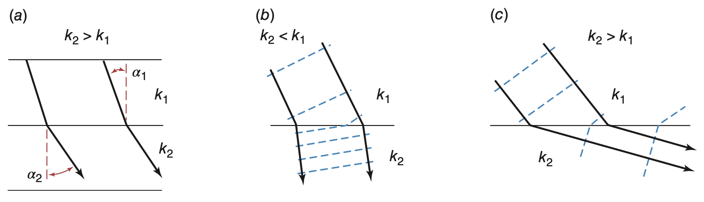
Two limiting cases are easy to remember:
- Into a much less conductive unit:
\alpha_2 \to 0 . The flow turns to cross the unit at right angles (straight down for a horizontal layer). - Into a much more conductive unit:
\alpha_2 \to 90° . The flow turns to run along the unit.
What refraction means in the field
Into the shale. Use the layered example again. Water in the sandstone that meets the boundary at 45° enters the shale at
Whatever the direction of flow in the sandstone, the water crosses the shale vertically. This is why cross sections show vertical arrows through every confining bed, and why flow through a confining bed can be treated as one-dimensional.
Into the sandstone. In the opposite case, the flow turns until it is nearly parallel to the bedding. A thin permeable bed therefore collects flow from the layers above and below it, and carries it sideways.
Together, these two results explain flow in layered ground. Water flows sideways in the conductive units and vertically through the less conductive units between them. Next week’s lecture covers these units in more detail.
The cross section at the end of this lecture shows both results: the flow arrows bend as they cross the contact.
Mapping a flow system
Potentiometric surface maps
- A potentiometric surface is an imaginary surface formed by the levels to which water rises in wells screened in one aquifer (Meinzer, 1923). A map of this surface is a contour map of hydraulic head.
- Two conditions must hold for the map to be meaningful.
- One aquifer. A deeper or shallower unit at the same place can have a very different head, as the piezometer nest showed. You must know which unit each well is screened in.
- Horizontal flow in the aquifer. Then equipotential lines are vertical and head does not change with depth. The depth and length of a well’s screen then do not affect the reading.
- Contour spacing shows the gradient. The head difference between contours is fixed, so close contours mean a steep gradient and widely spaced contours mean a gentle one.
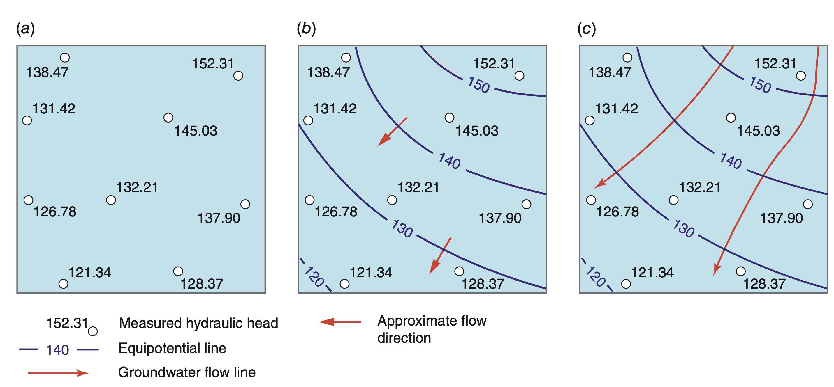
Three steps: plot the measured heads, draw contours, then add arrows at right angles to the contours, pointing towards lower head.
Three warnings about these maps
A potentiometric surface is not a water table
For an unconfined aquifer the two are the same, because the top of the saturated zone is the water table.
For a confined aquifer the potentiometric surface is above the top of the aquifer, often far above. It shows the level to which water would rise in a well. There is no water at that level in the ground.
Where the potentiometric surface is above the ground surface, a well flows without pumping. This is an artesian bore, and the Great Artesian Basin is named after them.
Right angles are an assumption
Flow arrows are drawn at right angles to the contours. This is correct only in isotropic material.
In layered ground, which is most ground, the flow direction turns away from the right angle, towards the direction with higher conductivity.
- A third, practical warning: all the measurements on one map must be taken at the same time. Heads change by metres from season to season. A map made from readings spread over a year mixes seasonal changes with differences between places.
Example: the Memphis aquifer
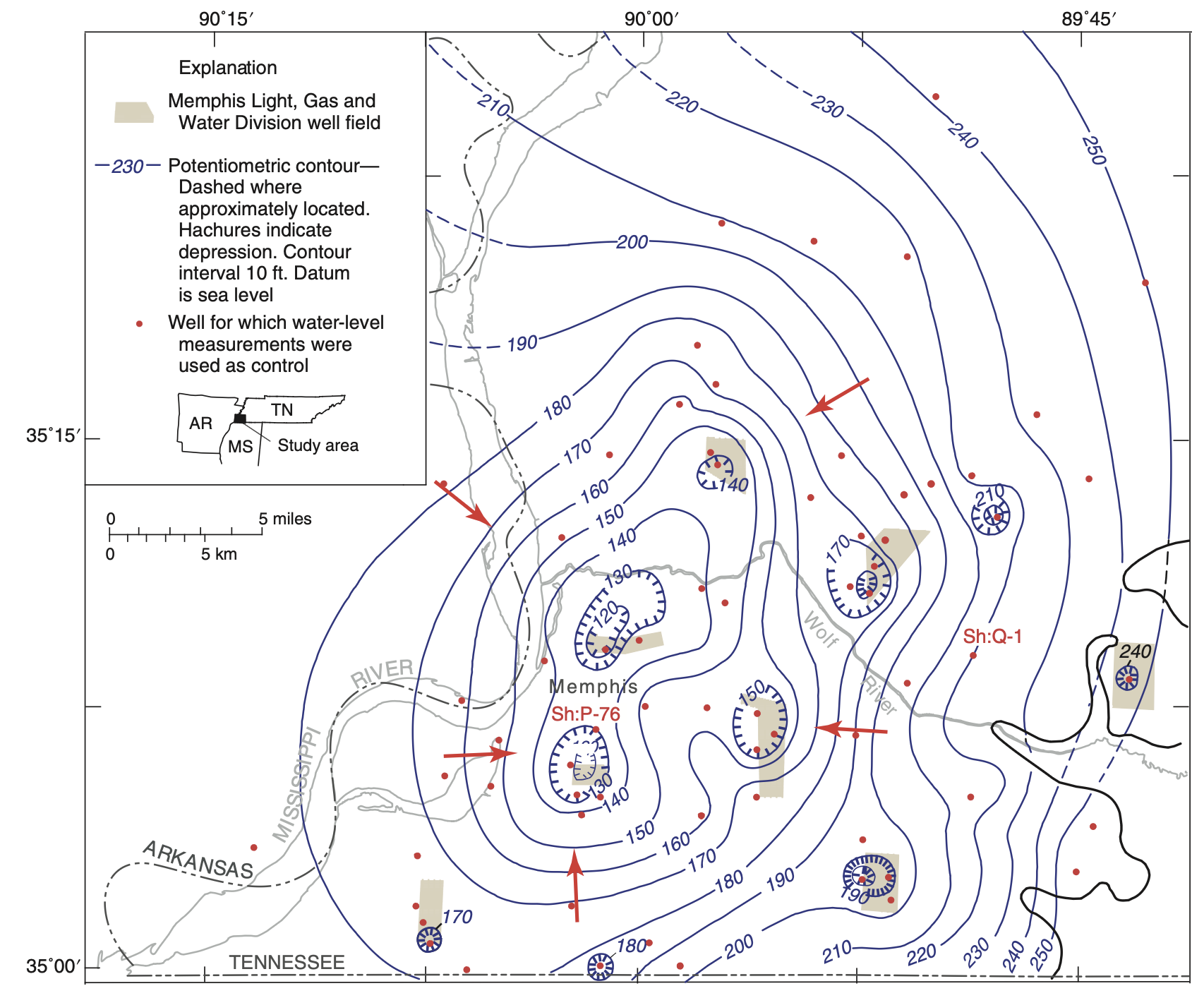
- The Memphis Sand in 1995, contoured from wells screened only in that unit.
- Each well field produced a local cone of depression. The cones overlapped and merged into one regional low in the centre of the map.
- Around the low the contours are close together, so the gradient is steep, and all flow arrows point inward. Most of the water that once flowed to natural outlets now flows to the pumps.
- Pumping was later reduced, and the water levels stopped falling. The hydrograph on the next slide shows this.
Water-level hydrographs
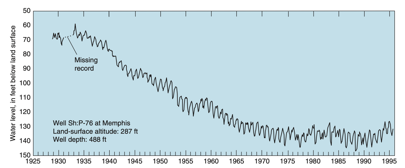
- A water-level hydrograph is a plot of head at one well against time. A map shows many places at one time. A hydrograph shows one place over a long time.
- In the past, someone measured each well monthly with a tape. Today, loggers record the level and send it over satellite or mobile networks.
- Well Sh:P-76 in the Memphis aquifer was monitored from 1925 to 1995. Its level falls steadily for forty years, then stays level from about 1970, when pumping was reduced.
- What to look for in a hydrograph:
- Seasonal cycle: recharge in the wet season, drawdown from irrigation pumping in the dry season.
- Trend: the long-term balance between recharge and pumping.
- Steps: a new well field, a new allocation rule, a drought.
- Maps of past conditions are usually impossible to make, because nobody measured enough wells at the same time. Often a long record at one well is the only data available.
Hydrogeological cross sections
- A cross section is a vertical slice through the flow system. It is drawn along the main flow direction, so that little flow crosses the plane of the section.
- It shows the rock layers, the conductivity of each unit, the heads measured in piezometer nests along the line, and the equipotentials drawn from them.
- In the example, a low-
K unit lies above an aquifer. In the upper unit, flow is nearly vertical and the equipotentials are close together, so the gradient is steep. In the aquifer, the equipotentials are vertical, and flow is horizontal with a gentle gradient. At the contact, the flow lines refract. - The vertical scale is exaggerated to make the layers visible. On an exaggerated section, flow lines and equipotentials do not meet at right angles, although they are often drawn that way.
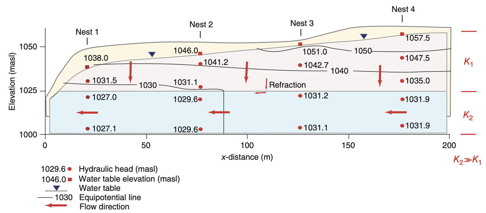
This figure brings together the main ideas of this lecture: heads measured at points, a gradient, two conductivities, refraction, and the flow direction that results from them.
Measuring groundwater storage from space
Ground measurements sample small volumes
- A piezometer samples a volume a few metres across. A pumping test samples a few hundred metres. A basin is hundreds of kilometres across.
- Head is not a volume of water. To convert a change in head to a change in volume, you need the storage properties from next week’s lecture, and these are rarely known well.
- Bores are not spread evenly over an aquifer. They are where someone needed water and paid for drilling: near towns, irrigation and roads.
- So adding up bore records cannot answer the basin-scale question: did this basin gain or lose water this decade?
Since 2002, satellites have answered this question directly. Water has mass, so a change in stored water changes the gravity field, and satellites can measure that change.
The size of the signal
The Millennium Drought removed about 140 km³ of water from the Murray-Darling Basin.
Spread over the basin’s
GRACE detects this 13 cm change from an altitude of about 490 km.
How GRACE measures water mass
- Two identical satellites fly in the same orbit at about 490 km altitude, one about 220 km behind the other.
- A microwave link measures the distance between them continuously, to within a few micrometres.
- When the pair approaches a region of extra mass, the leading satellite is pulled forward first, and the distance increases. When the trailing satellite reaches the mass, the distance decreases again. A month of these distance changes is used to calculate a map of the global gravity field.
- Mass changes that are not water are calculated with models and removed: the atmosphere, ocean tides, and the slow rise of the crust since the last ice age. Over Australia the last correction is small, which makes Australia a good place to use GRACE.
- The result is given as equivalent water thickness, in millimetres of water, as the difference from the mean of a reference period.
What the measurement can and cannot resolve
- Each monthly gravity field is a sum of spherical harmonics up to about degree 50. This resolves features of about 400 km on the ground. Newer mass concentration (mascon) solutions come on finer grids, but the true resolution is still about the same.
- So GRACE can resolve large basins. It cannot resolve individual farms or bores. Published studies use areas of at least
10^{5} to10^{6}\ \mathrm{km^2} . - The Murray-Darling Basin, at
1.06\times10^{6}\ \mathrm{km^2} , is close to the smallest area that GRACE can resolve with confidence. GRACE cannot resolve the Murrumbidgee catchment on its own. - Mass changes outside the basin appear in the basin estimate, and mass changes inside the basin appear outside it. This is called leakage, and correcting for it is most of the work in a GRACE study.
Three more limitations
- No depth information. Gravity gives the change in mass of a whole column. It cannot tell whether the water came from a reservoir, the soil or an aquifer 200 m down.
- One value per month at best. Individual storms and recharge events are not visible.
- A gap in the record. GRACE ran from 2002 to 2017 and GRACE-FO began in 2018. The eleven months between them are missing from every time series.
In return, GRACE gives something that no network of bores can: a monthly total for the whole basin, over twenty years, that does not depend on where bores were drilled.
From total storage to groundwater
Gravity measures all the water in the column at once:
To get groundwater, subtract the other stores, each estimated from a separate data source:
- Surface water comes from reservoir and river records. Soil moisture comes from a land surface model or from satellites. Snow is negligible in the Murray-Darling Basin.
- Every error in these terms goes into the groundwater estimate. The groundwater estimate is therefore only as good as the soil moisture estimate.
Does the subtraction work?
Leblanc et al. (2009) tested it over the Murray-Darling Basin against ground measurements.
- Annual GRACE storage against the sum of measured groundwater, surface water and soil moisture: R = 0.94.
- GRACE minus soil moisture and surface water, against measured groundwater alone: R = 0.92.
The groundwater estimate from GRACE agrees well with the bore measurements.
Assignments II and III ask you to do this calculation, with the CSR mascons for total storage and the ESA CCI record for soil moisture.
The Millennium Drought seen by GRACE
Murray-Darling Basin, 2001 to 2007, from Leblanc et al. (2009):
| Store | Change | Over what period |
|---|---|---|
| Soil moisture | 2001 to 2003 | |
| Surface water | 2001 to 2003 | |
| Groundwater | 2001 to 2007 |
- Average total deficit over the GRACE record: 140 km³. Peak deficit, January to March 2007: 240 km³.
- Soil moisture and surface water fell within two years, and then stopped falling because little was left. Groundwater was still falling after six years.
- Rainfall returned to average in 2007. Groundwater storage did not recover.
What the sequence shows
A drought moves through the water stores in order of their residence times. Rainfall falls first, then soil moisture within months, then streamflow, then groundwater over years. Groundwater also recovers last.
By the rainfall record, the drought ended in 2007. By groundwater storage, it had not.
- This is why we measure storage directly, instead of estimating it from rainfall.
- Earlier parts of this lecture explain why groundwater responds slowly: low
K , long flow paths, and residence times of decades.
What we learned
- Porosity and conductivity are different properties. Porosity tells you how much water the ground holds. Conductivity tells you how fast the water flows. Clay has one of the highest porosities and one of the lowest conductivities.
- Head sets the direction of flow.
h = z + P/\rho_w g . In still water, head is constant but pressure is not. Head belongs to a point, so one site can have several heads. - Darcy’s law,
q = -K\,dh/dl , was found by measurement, and the pore scale explains it:K \propto d^2 \rho_w g/\mu . This result explains the range ofK from gravel to clay, the grain-size formulas, and the split ofK into permeability and fluid properties. - Divide
q by the effective porosity to get the speed of the water. In fractured rock, the water can travel a hundred or more times faster thanq . - Layering turns heterogeneity into anisotropy. Along the bedding, use the arithmetic mean: the most conductive layer controls
K_h . Across the bedding, use the harmonic mean: the least conductive layer controlsK_v . Isotropic layers alone can giveK_h/K_v = 10^6 . - Flow lines refract at a contact. They cross a less conductive unit at right angles, and turn to run along a more conductive one.
- Field methods: piezometer nests for vertical gradients, potentiometric maps for one aquifer at one time, hydrographs for change over time, and GRACE for the whole basin.
Next week: aquifers. The different types of aquifer, and how much water they release when the head falls.