- / -
EMSC3025/6025: Remote Sensing of Water Resources

Precipitation
EMSC3025/6025
Dr. Sia Ghelichkhan
Objectives
Introduce the role of precipitation in the hydrological cycle.
Understand how precipitation forms in the atmosphere.
Explore factors controlling the amount and distribution of precipitation.
Examine how vegetation interacts with and modifies precipitation.
Review methods for measuring and estimating precipitation.
Understand how radar and satellite remote sensing estimate rainfall over an area, and where they fail.
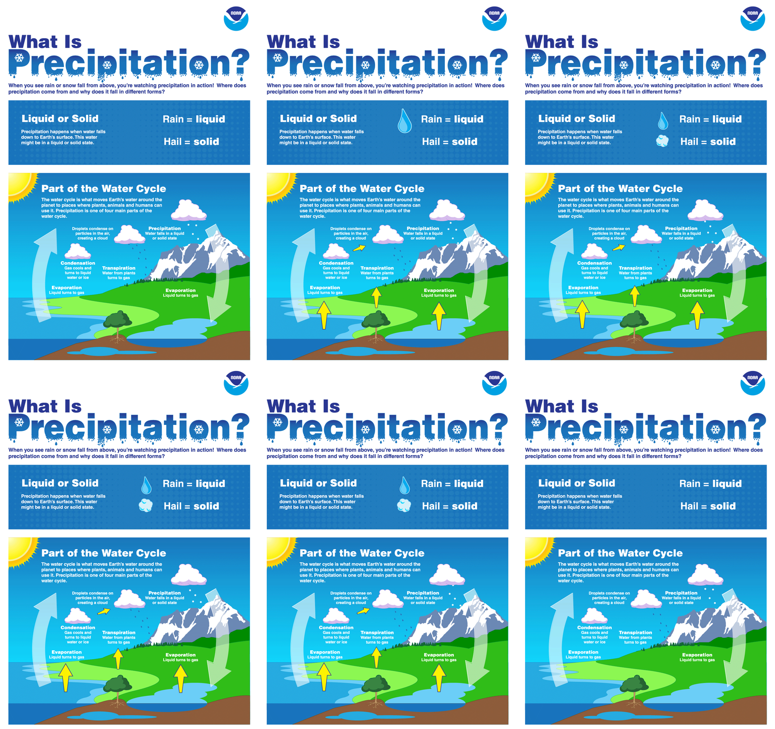
Fig. 1 → From scijinks.gov
Precipitation
The release of water from the atmosphere to reach the surface of the Earth.

- Covers all forms of water: snow, hail, sleet, and rainfall.
- The ability of air to hold water vapour is temperature dependent.
Understanding the Atmosphere
Before we can understand precipitation, we need to understand the atmosphere, or more specifically:
What causes the air to cool?
Composition of the Atmosphere
Let’s understand pressure and temperature relationships first.
- Atmosphere around us is a mixture of gases
- Nitrogen and oxygen make up 99% of the atmosphere (plus some water vapour)
- Gravity keeps the atmosphere close to the surface, hence the pressure is higher at the surface.
- e.g., at 5500m elevation, the pressure is 50% of the surface pressure.
- Units
[Pa] = N \, m^{-2} , but commonly reported in[millibars] or[kPa] - Water vapour accounts for
< 0.3 \% of the atmospheric pressure.
pie showData
    "Nitrogen" : 78
    "Oxygen" : 21
"Other gasses, including water vapour" : 1Cooling of the atmosphere
- Moist Air = Water vapour + Dry air
- The maximum amount of vapour that air can hold depends on the temperature.
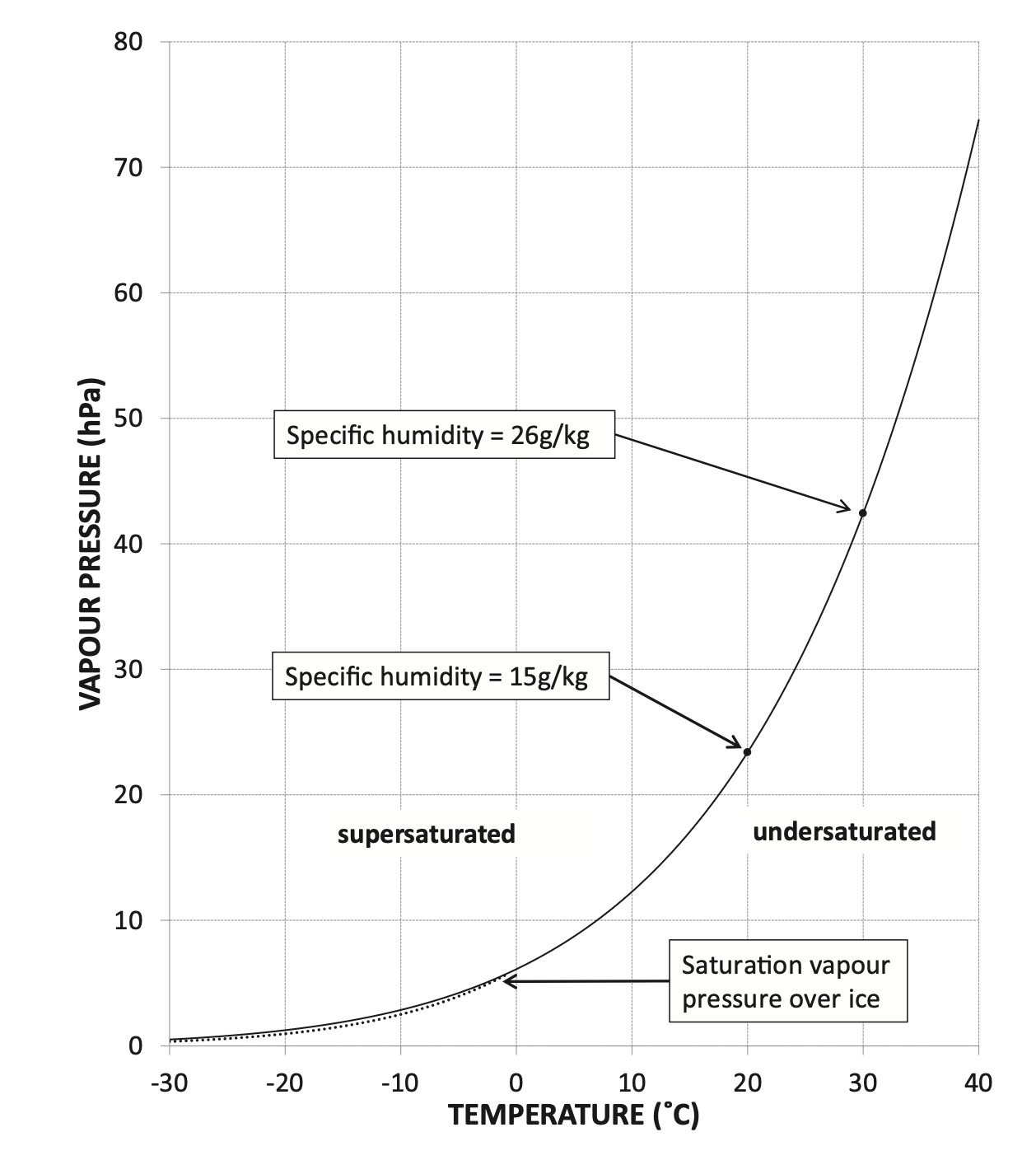
- Clausius-Clapeyron equation describes the relationship between temperature and vapour pressure.
- Figure 2 →
Saturation vapour pressure curve representing absolute humidity for a given dew point temperature. Note that the saturation vapour pressure curve over ice is lower.
Cooling of the atmosphere
- Vapour pressure
e(T) , cannot exceed saturated vapour pressuree_{sat} . e_{sat} represents absolute humidity: the vapour pressure at which vapour starts to condense into liquid.- The temperature at which a parcel reaches
e_{sat} is its dew point temperature (frost point temperature below 0°C). - We could also have super-saturated air, where the vapour pressure is higher than the saturated vapour pressure (maximum 1 or 2%).
- The dotted line represents the saturation vapour pressure curve over ice.
- Easier to escape from the liquid phase to the vapour phase compared to the solid phase.
- Subzero temperatures: where desublimation occurs. (hoarfrost).
Cooling of the atmosphere
- Vapour Pressure is a reflection of the concentration of water vapour molecules in air.
- Specific humidity: mass of water vapour (g) per unit mass of air (kg).
- Temperature increase of 10°C allows air to hold ~11g more water vapour per kg of air.
- Example: At 30°C vs 20°C:
- 30°C: 26 g water vapour per kg air
- 20°C: 15 g water vapour per kg air
Adiabatic Cooling and Lapse Rates
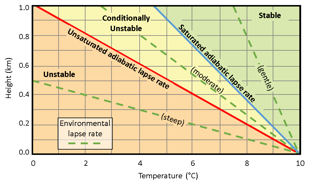
- Adiabatic cooling: When air moves upward to lower pressure, it expands and cools.
- Cooling occurs due to pressure and density changes, not heat loss.
- Fundamentally important in precipitation formation process.
- Dry Adiabatic Lapse Rate (DALR): ~9.8°C per km for dry air.
- Saturated Adiabatic Lapse Rate (SALR): Slower than DALR due to latent heat release from condensation.
- SALR can be half the DALR - precise value depends on pressure and temperature.
Environmental Lapse Rate
- Environmental Lapse Rate (ELR): Conventional temperature decrease with altitude.
- Related to distance from radiating body (Earth).
- Approximately 6°C per km, but varies.
- Three types of lapse rates:
- DALR: ~9.8°C/km (dry air)
- SALR: ~4-6°C/km (saturated air, varies)
- ELR: ~6°C/km (environmental, varies)
Adiabatic cooling process
Now we understand the atmosphere, but how does precipitation form?
Three physical conditions must be met for precipitation to occur:
- Cooling of the atmosphere
- Condensation onto atmospheric nuclei
- Growth of water/ice droplets large enough to overcome updrafts
- a supply of moisture to continue the process
How do we cool the air?
- Cooling is essential for condensation and precipitation:
- Rising air moves to lower pressure, expands and cools
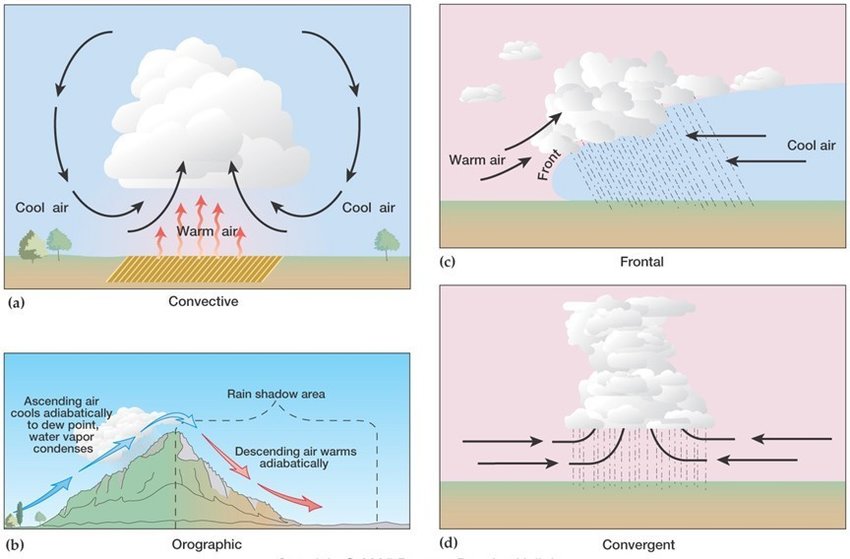
- Main causes of uplift:
- Convective: surface heating
- Orographic: air rising over mountains
- Cyclonic: air lifted in low-pressure systems
- Also caused by contact with cooler surfaces or air masses
Condensation Nuclei
- Minute particles (1
\mu m ), initiating droplet formation. - surface for vapour to condense into liquid.
- Include dust, smoke, sea salt
- Without them, supersaturation can occur without precipitation
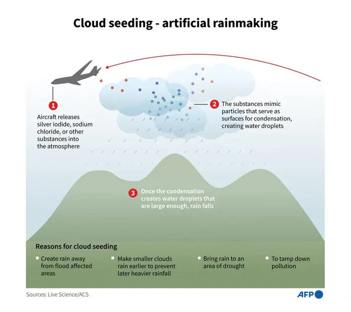
- Forms a basis for cloud seeding (silver iodide, more recently potassium chloride)
- Various forms of cloud seeding: References (Mather et al. 1997)
- Case of a paper mill in South Africa.
Droplet Growth Processes
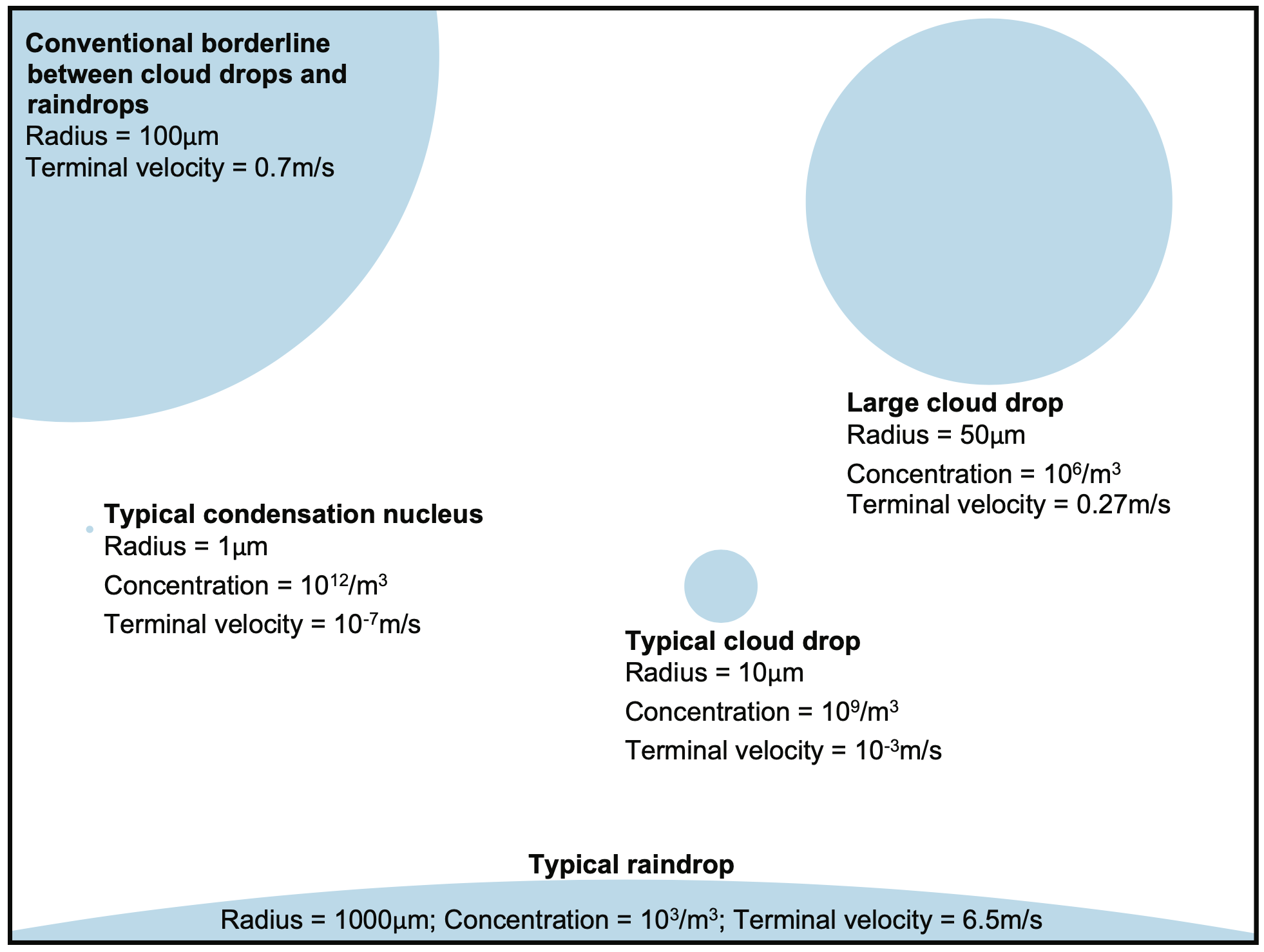
- Water/ice droplets need to be large enough for them weight to overcome upward draught (from a cloud).
- They need to grow from
\approx 1\mu m to\approx 3000\mu m .
Droplet Growth Processes
- Difference in vapour pressure and water ⇒ vapour adds to droplets (slow)⇒ Condensation on water.
- Difference in pressure with ice bigger ⇒ faster, due to greater vapour gradient Sublimation on ice.
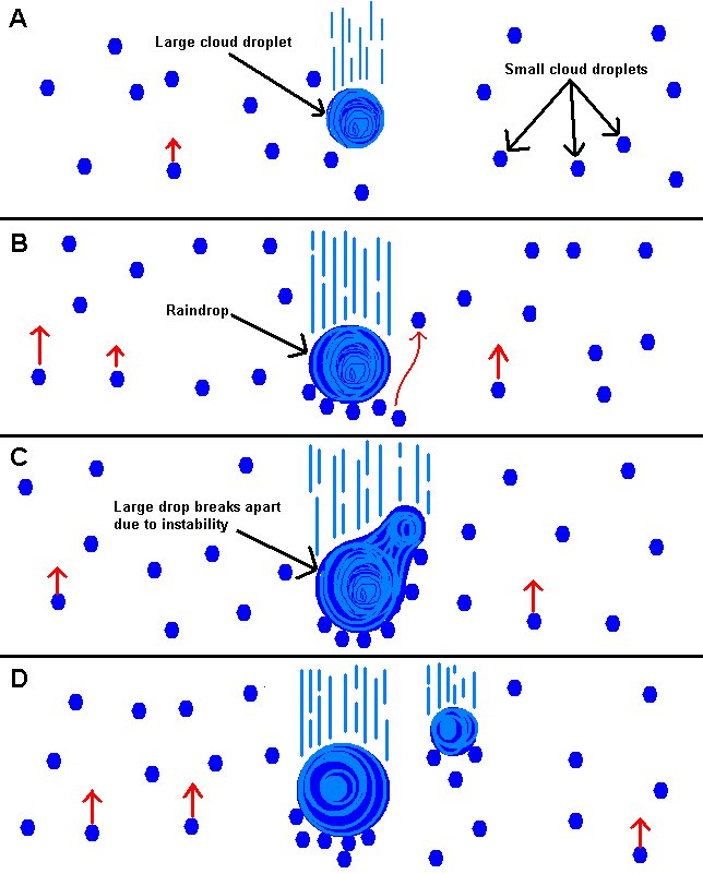
- Main process that raindrops grow: Collision and coalescence, two water-drops collide and join together and they repeat.
- Dominant in warm clouds.
- Droplets collide, merge, and grow large enough to fall.
- Larger droplet fall faster, sweep a larger area and are more likely to collide with other droplets.
- When ice droplets grow by collision, it’s called aggregation.
Different types of clouds
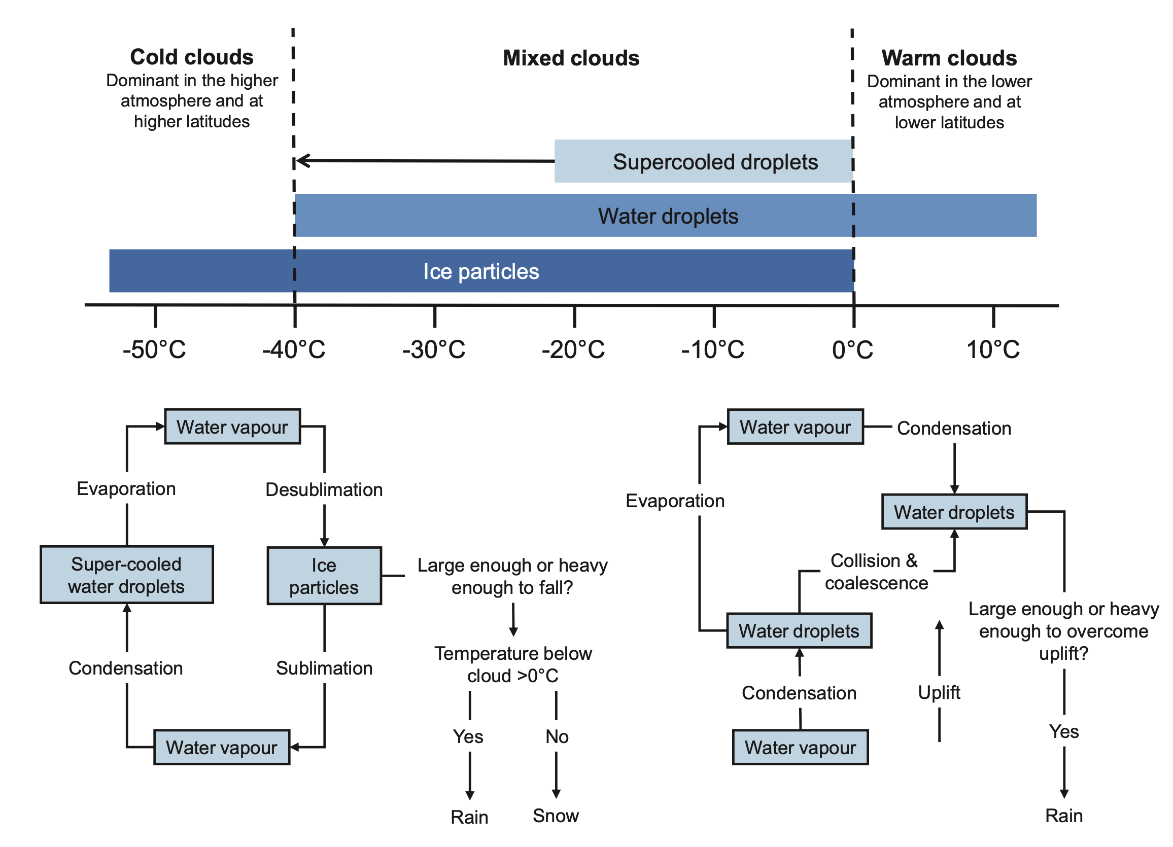
Bergeron Process
- Bergeon-Findeisen Process or cold cloud process.
- At sub zero temperatures, the saturation vapour pressure over ice is lower than over water.
- This means air is saturated for ice but not for water.
- Which means the ice particles can grow at the expense of the water droplets.
- Vapour diffusion: vapour moves from higher pressure (cloud droplets) to lower pressure (ice particles).
- But this results in drier clouds ⇒ cloud droplets evaporate.
- Ice particles attract water vapour efficiently, causing desublimation (direct vapour to ice).
Hail Formation
- Hail stones: typically ~5mm, spherical, sometimes irregular ice particles.
- Size range: golf ball size common, rare cases >15cm diameter recorded.
- Formation location: highest parts of cumulonimbus clouds (storm clouds).
- Process: ice particles circulate in violent up/down draughts.
- Growth mechanism: ice particles collide with supercooled water droplets → immediate freezing.
- Cross-section: alternating layers of clear and translucent ice.
- Clear ice: slower freezing (cloud tops)
- Translucent ice: instant freezing, trapped air
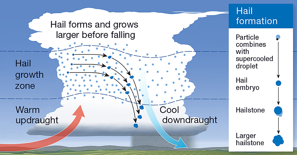
Hail Formation Process
- Circulation: hail stones circulate multiple times in violent draughts.
- Fall mechanism: increasing mass eventually overcomes up draught.
- Melting: if conditions warmer below cloud base → melt and fall as rain.
- Damage potential: serious damage to infrastructure and agriculture.
- Economic impact: US hail storms cause ~$1 billion/year in losses.
- Reference: National Storm Damage Centre
Precipitations and Definitions
| Class | Definition |
|---|---|
| Drizzle | A subset of fine rain with droplets between 0.1 and 0.5 mm, but close together |
| Rain | Liquid water droplets with diameter between 0.5 and 0.7 mm, but smaller if widely scattered |
| Freezing rain or drizzle | Rain or drizzle, the drops of which freeze on impact with a solid surface. Also called sleet in the USA |
| Sleet | Partly melted snowflakes, or rain and snow falling together (UK). Fairly transparent grains or pellets of ice (USA) |
| Ice crystals, ice prisms, snow and snowflakes | Snow can fall as single branched hexagonal or star-like ice crystals, or in the case of ice prisms, as unbranched ice crystals in the form of hexagonal needles, columns or plates. The nature of the crystal depends on the temperature at which it forms and the corresponding amount of water vapour. More often snow falls as agglomerated snowflakes. |
| Snow grains | Very small, white, opaque grains of ice, flat or elongated, with diameter generally <1 mm. Also called granular snow |
| Snow pellets | White, opaque grains of spherical or conical ice (2–5 mm). Also called granular snow, or graupel |
| Ice pellets | Transparent or translucent pellets of ice, spherical or irregular with diameter <5 mm |
| Hail | Balls or pieces of ice usually between 5 and 125 mm in diameter, commonly showing alternating concentric layers of clear and opaque ice in cross-section |
Understanding spatial distribution
We understood the process, but we need to understand how precipitation is distributed mostly in space
Precipitation Distribution
Precipitation varies across both space and time:
- Spatial variation: different locations receive different amounts.
- Temporal variation: amount of rainfall changes over time at the same location.
Influences on precipitation fall into two categories:
- Static influences: do not change from storm to storm (e.g. altitude, aspect, slope)
- Dynamic influences: change with weather conditions (e.g. air masses, storm tracks)
Higher rainfall in the north-west states (Oregon and Washington) due to linked to wetter cyclonic weather systems from the northern Pacific. Higher rainfall in Florida and other southern states is linked to the warm waters of the Caribbean sea
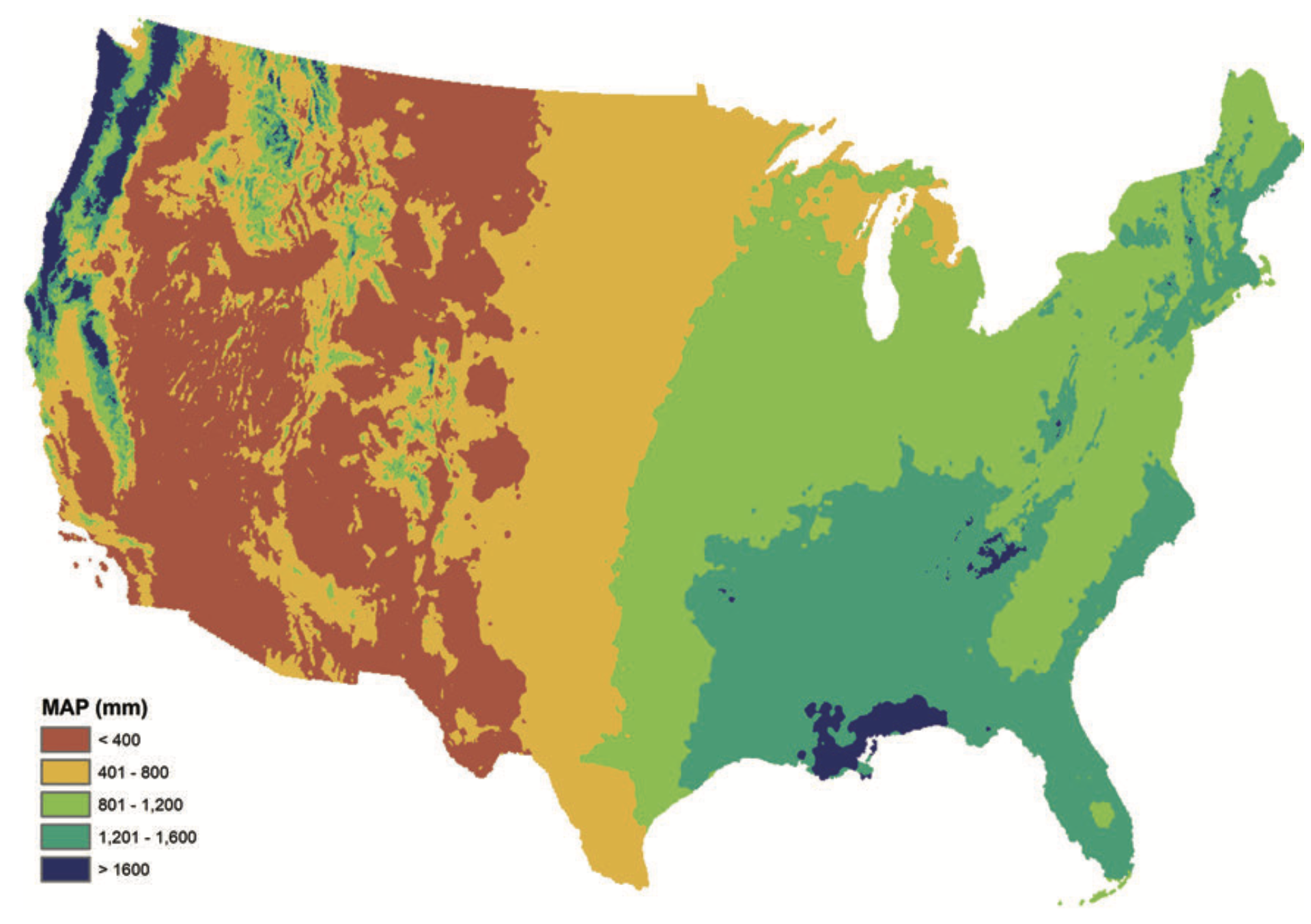
Static Influences on Precipitation
flowchart LR
    A([Precipitation]) --> B([Dynamic Controls])
    A --> C([Static Controls])
    C --> D([Altitude])
    C --> E([Aspect])
    C --> F([Slope])

    classDef bigText font-size:28px;
class A,B,C,D,E,F bigTextStatic influences are fixed features of the landscape:
- Altitude: Modulating temperature. Higher elevations receive more rainfall due to cooling of rising air (orographic effect)
- Aspect: Less important than altitude. Slopes facing prevailing winds often receive more precipitation.
- Humid mid-latitudes (35-65
\degree ): cyclonic weather systems coming from W. So slopes facing east will be more sheltered.
- Humid mid-latitudes (35-65
- Slope: Only important at very small scale – i.e., the difference between a level gauge and one on a slope.
Case Study: The rain shadow effect
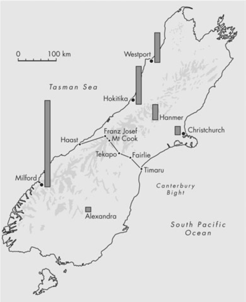
Predominant weather pattern for the South Island of New Zealand is a series of rain-bearing depressions sweeping up from the Southern Ocean, interrupted by drier blocking anticyclones.
Weather pattern: westerly airflow, bringing moist air from the Tasman Sea.
One the west side, mostly rain. On the eastern side: föhn (locally as nor-wester).
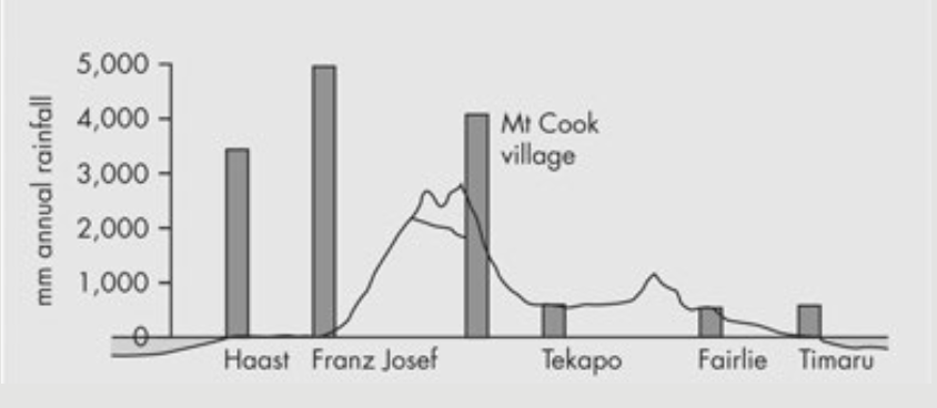
Rainfall distribution across the Southern Alps of New Zealand (South Island). Shaded areas on the map are greater than 1,500 m in elevation. A clear rain shadow effect can be seen between the much wetter west coast and the drier east
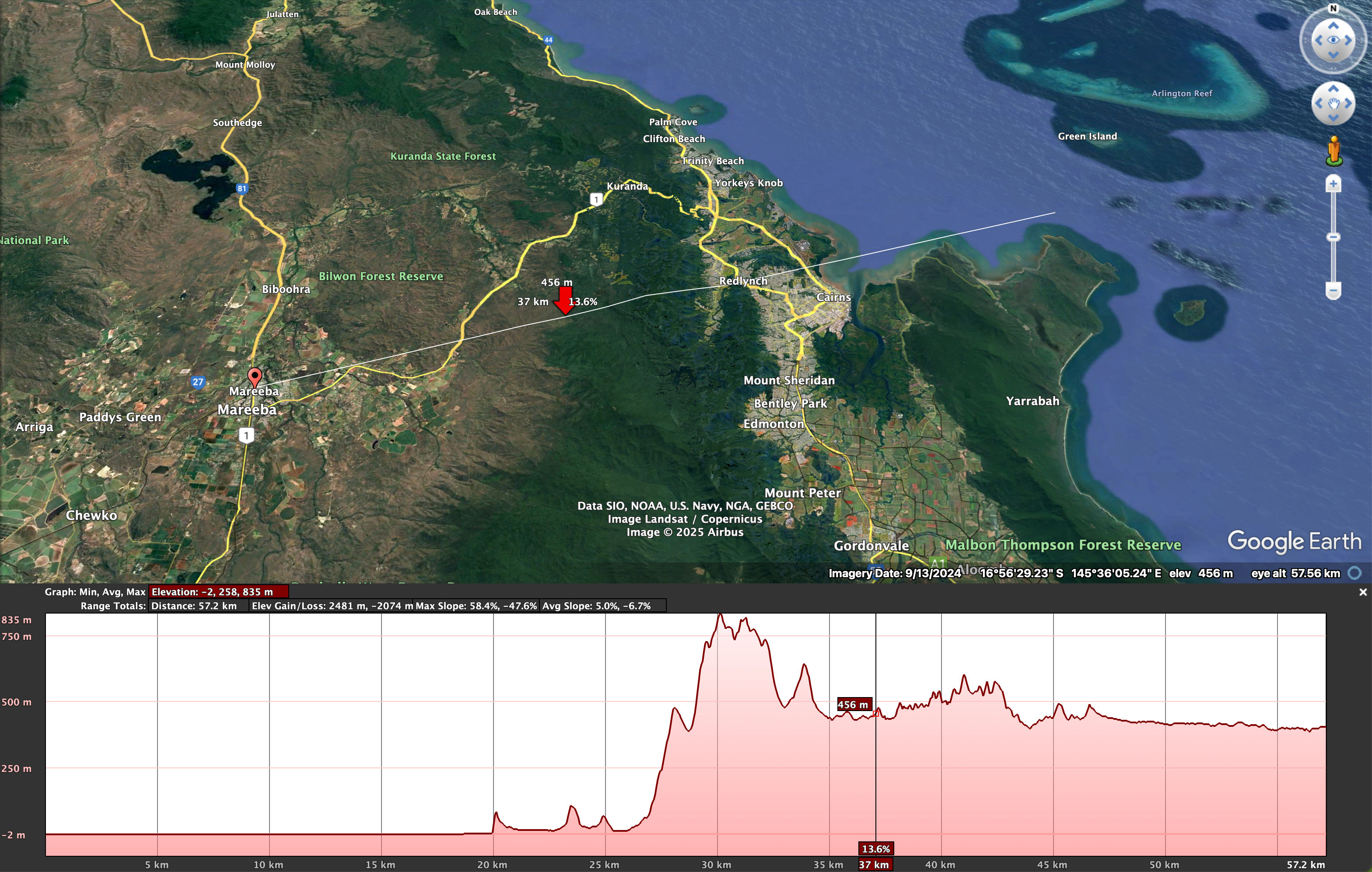
Case Study: The rain shadow effect in Mareeba
Case Study: The rain shadow effect in Mareeba
Dynamic Influences on Precipitation
Dynamic influences result from atmospheric processes (climatic controls) that vary with time:
Storm tracks: paths of cyclones and weather systems
Frontal systems: interactions between warm and cold air masses
Moisture availability: seasonal shifts in humidity sources (e.g. monsoons)
Convective activity: varies by temperature and surface conditions
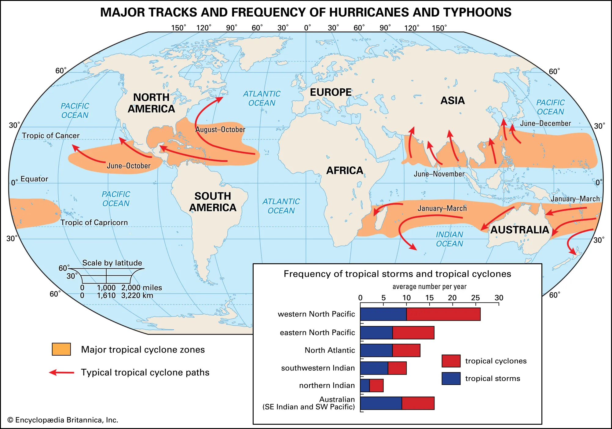
At the global scale, dynamic factors dominate:
- Climate zones
- Atmospheric circulation (e.g. ITCZ, subtropical highs)
At the continental scale, both static and dynamic factors matter:
- Mountain ranges cause rain shadow effects
- Seasonal wind and temperature patterns affect rainfall distribution
Measurement of Precipitation
How do we measure precipitation?
Measurement of Precipitation
Measured as a vertical depth of water (e.g. mm or inches).
Represents the depth that would accumulate if all water remained on the surface.
Used for both rain and snow:
- Snow is often reported as water equivalent.
- Recognizes that snow can occupy up to 90% more volume than liquid water.
Due to spatial variability, there’s a strong argument that catchment-scale precipitation cannot be “measured.”
Thus, all precipitation “measurement” techniques are effectively estimation techniques.
For clarity in this course:
- Measurement: quantifies actual water collected.
- Estimation: uses surrogate variables (e.g., radar, satellite).
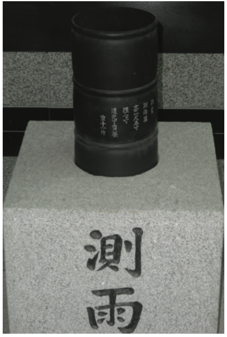
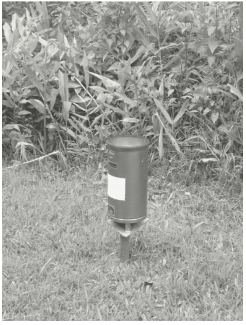
Rainfall Measurement with Gauges
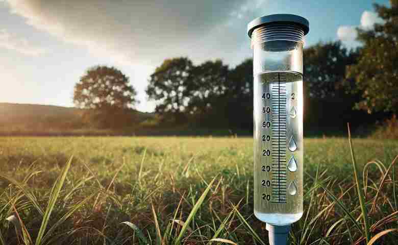
- Rain gauge: collects rainfall over a defined area, measures volume.
- Volume is divided by the area to get depth.
- Simple in concept — but prone to multiple sources of error.
Errors in Rainfall Measurement
flowchart TB
    A([Rainfall Measurement Errors]) --> B([Evaporation])
    A([Rainfall Measurement Errors]) --> C([Wetting])
    A([Rainfall Measurement Errors]) --> D([Rain Splash])
    A([Rainfall Measurement Errors]) --> E([Turbulence])

    classDef bigText font-size:28px;
        class A,B,C,D,E,F bigText
Four major sources of error:
- Evaporation: water lost before being measured.
- Wetting: water adheres to funnel walls.
- Rain splash: water splashes into or out of the gauge.
- Turbulence: wind distorts drop paths, reduces catch.
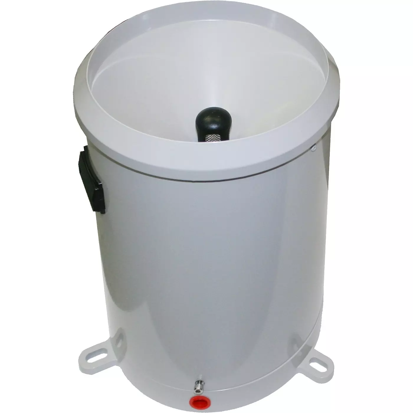
Evaporation Loss
- Funnel-shaped design channels water to a narrow opening.
- Reduces air mixing and exposure to sunlight.
- Minimizes evaporative losses by:
- Preventing warm air exchange
- Shading the collected water
- Evaporation is limited if turbulence is reduced (more in Chapter 3).
Wetting Loss
- Water clings to funnel walls and may not reach the collector.
- Losses are usually small, but significant during:
- Light showers
- Warm days
- Solutions:
- Steep funnel sides
- Non-stick surfaces (e.g., copper or non-adhesive plastics)
Rain Splash
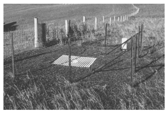
- Ideal gauge would sit flush with the ground — but this increases splash-in.
- Funnel design prevents splash-out, creating a net over-measurement.
- Surface-level gauges may flood or be covered by snow.
- Raised gauges or non-splash surrounds are preferred.
Wind Turbulence and Gauge Height
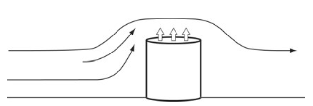
- Raised gauges reduce splash, but disrupt airflow.
- Wind creates turbulent eddies, leading to under-catch.
- Loss increases with:
- Wind speed: At 20 km/h: up to 20% loss, at 90 km/h: up to 40% loss
- Drop size
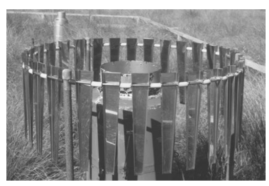
- Solution: fit gauge with a wind shield (e.g. baffles or slats).
- Shields reduce wind speed around the orifice.
- Can significantly improve measurement accuracy.
Rain measurement in Australia
No universal “perfect” design.
The best gauge depends on:
- Local conditions (e.g. snow, wind exposure)
- Practical installation needs
The non-splash grid + surface-level gauge is closest to ideal:
- Reduces splash and turbulence
- Unsuitable for snow-prone areas (risk of burial)
The standard rain gauge in Australia is a 203 mm manual gauge, which collects rainfall into a graduated cylinder.
It is mounted 0.3 m above the ground, away from obstructions.
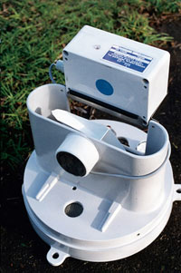
Modern stations use Tipping Bucket Rain Gauges (TBRG):
- Each tip = 0.2 mm of rain
- Measures rainfall intensity and rate
- Snow gauges are used in alpine areas with melt tanks or antifreeze methods.
- Readings are mostly taken at 9am daily, often by volunteers.
- Rainfall is recorded to the nearest 0.2 mm or 0.1 mm in recent years.
Challenges of Measuring Snowfall
- Snow measurement faces greater errors than rainfall:
- Snowflakes are easily transported by wind before and after settling.
- Leads to drifting and uneven surface distribution.
- Raindrops, by contrast, rarely redistribute after hitting the ground.
- Measurement errors resemble rain splash but more extreme.
Two main approaches:
- Snow gauges (modified rain gauges)
- Ground snow depth measurements
Both suffer from:
- Wind transport and drift
- Uneven accumulation
- Sampling errors (point measurements ≠ area representation)
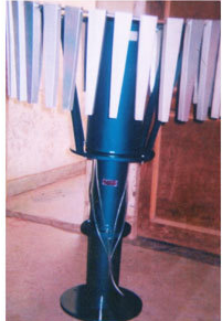
Rain Gauge Modification for Snow
Modifications needed to measure snow with a rain gauge:
- Heated rim melts falling snow into water
- Prevents snow buildup and overflow
- Requires power supply — impractical in remote areas
- Drainage system must move water away from heat source
- Prevents evaporation losses
- Raised gauge keeps instrument above snow surface
- Increases turbulence error
- Typically paired with wind shields or deflectors
Measuring Snow Depth: Core Sampling
- Core sampler:
- Extracts a vertical column, measures depth and density
- Snow is then melted to determine water equivalent depth
- Limitations:
- Point-based, non-continuous measurementm; location-dependent: snow drift and exposure affect accuracy
- Similar in limitation to daily manual rain measurements
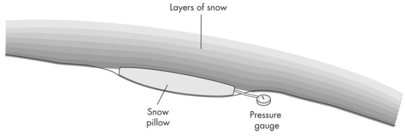
- Snow pillows measure accumulated snow mass
- Capture snowpack water storage, not just depth
- Used in hydrology for estimating delayed runoff
From point measurements to spatial rainfall estimation
- Rain gauges provide rainfall data at specific points.
- Hydrologists, however, need to know rainfall over a whole catchment.
- This requires converting point data into areal estimates using spatial averaging techniques.
- Factors influencing rainfall distribution:
- Gauge density and placement
- Topography (e.g. elevation, slope)
- In practice, we apply methods to estimate catchment-wide rainfall from gauge networks.
- These methods will be covered in the tutorials.
Thiessen Polygons
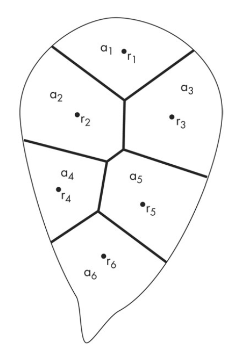
- American engineer Thiessen (1911) developed a method to overcome uneven distribution of rainfall gauges.
- Attach an area to each gauge. Every point in the area is closer to that gauge than any other gauge.
- Connect each gauge to its nearest neighbours.
- Find the perpendicular bisector of the line segment connecting the two gauges.
- Extend the bisectors until they meet.
- Find the area associated with each gauge.
- Then:
R = \sum_{i=1}^{n} r_i \times \left(\frac{a_i}{A}\right) whereR is the areal rainfall,r_i is the rainfall at thei -th gauge,a_i is the area of thei -th polygon, andA is the total area of the catchment.
Hypsometric method
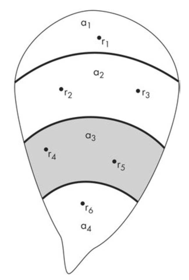
- It is well known that the altitude of the catchment (among other factors) affects the rainfall.
- Here we change the polygons into a hypsometric curves.
- That is we are assuming points with unknown rain measurements should have the same rainfall as the points with known rainfall at the same altitude.
Isohyetal method
- An isohyet is a contour of equal rainfall. Here we weight by the measured rainfall itself, not by a surrogate like altitude.
- Requires a large number of gauges: interpolate between the gauge values, draw the isohyets, then measure the area between each pair.
R = \sum_{i=1}^{n} r_i \times \left(\frac{a_i}{A}\right) where nowa_i is the area between two isohyets andr_i the average rainfall between them. - Same equation as Thiessen and hypsometric — only the definition of
a_i changes. - With the advent of computing, these techniques have improved a lot.
- e.g., kriging!
Same figure as before, but the bands are now contours of rainfall rather than of elevation
GIS, interpolation and geostatistics
- Thiessen / hypsometric / isohyetal are all weighted averages — done by hand, on paper.
- In a GIS we instead build a rainfall surface on a grid:
- Smoothing: the surface need not pass through the gauges (e.g. splines, multi-quadric).
- Interpolation: the surface does pass through them (nearest neighbour, inverse distance).
- Geostatistics goes one step further and uses the spatial correlation of the field itself.
- Nearby gauges are more alike than distant ones.
- Kriging: fit a semi-variogram describing how the difference between pairs of gauges grows with separation, then estimate unsampled points as a weighted average with weights derived from that variogram.
- Co-kriging brings in a second variable (e.g. elevation, or a radar field).
- Crucially, kriging also returns an uncertainty at every point — the other methods do not.
The problem of scale
- A rain gauge orifice is
\approx 0.03 \, m^2 . - A catchment is
10^6 –10^{12} \, m^2 . - We routinely scale up by ten orders of magnitude and call the result “the rainfall”.
- Clarke et al. (1973), Plynlimon, Wales: to get areal hourly rainfall to 90% accuracy over a 10 km² catchment needed
\approx 100 gauges. Four gauges gave\approx 50\% . - This is the motivation for everything that follows.
Surrogate measures: looking at the rain instead of catching it
If we cannot afford enough gauges, can we estimate rainfall from something we can observe over the whole area at once?
- Two families, differing fundamentally in which way they look:
- Radar: from the ground up into the cloud.
- Satellite: from space down onto the cloud top.
- Neither measures rainfall. Both measure electromagnetic radiation and convert it with a calibrated relationship.
- So both are estimation, in the sense we defined earlier — and both still need gauges, for calibration and for validation.
flowchart TB
    S([Satellite]) -- "sees cloud top: bright + cold" --> C([Cloud])
    C -- "sees hydrometeors inside" --> R([Ground radar])
    C --> G([Rain gauge: the truth, at one point])
    classDef bigText font-size:26px;
class S,C,R,G bigTextGround-based radar: the principle
- RAdio Detection And Ranging.
- A pulse of microwave energy is emitted; hydrometeors backscatter part of it.
- Two numbers come back:
- Return time
\rightarrow distance to the target,r = c \, t / 2 . - Returned power
\rightarrow reflectivityZ , i.e. how much water is in that volume.
- Return time
- Rotate the antenna in azimuth, step it in elevation
\Rightarrow a 3-D volume scan every 5–10 minutes. - Wavelength choice is a compromise:
- S-band (
\approx 10 \, cm ): barely attenuated by heavy rain, but needs a large dish. - C-band (
\approx 5 \, cm ): the usual operational choice, incl. most of Australia. - X-band (
\approx 3 \, cm ): cheap and portable, but attenuates severely.
- S-band (
- The wave must be reflected by liquid water, not by atmospheric gases or density gradients — this is why the band matters.
Reflectivity is not rainfall
Z weights drop diameter to the sixth power.- Rainfall rate weights it to roughly the third-and-a-bit power:
- So
Z andR are related, but only through the drop size distributionN(D) — which we do not know.
The Z–R relationship
- In practice we assume a power law:
- Marshall–Palmer:
a = 200 ,b = 1.6 — the default for stratiform rain. - Because
Z spans many orders of magnitude, it is reported logarithmically:
- Rules of thumb:
20 \, dBZ \approx drizzle,40 \, dBZ \approx 12 \, mm/hr ,>50 \, dBZ suggests hail. - The coefficients are not universal. Convective, stratiform, tropical and snow regimes each want different
a ,b . - Hence a radar must be calibrated against rain gauges, often over several years, at each site.
Worked example
A radar reports
Now use a tropical convective relation,
Nearly a factor of three, from the same measurement. This is the central weakness of radar QPE.
Why radar rainfall goes wrong
- Drop size distribution: as above — one
Z , many possibleR . - The bright band: melting snowflakes are large and water-coated, so they are highly reflective. The radar sees a bright ring at the melting level and over-estimates rain by up to a factor of five.
- Beam blockage: hills between the radar and the storm remove part of the beam. A permanent, terrain-fixed bias.
- Beam broadening and overshoot: the beam widens with range (
\approx 1° ), so at 150 km it samples a\approx 2.5 \, km deep layer, high above the ground — and may pass clean over shallow orographic rain. - Attenuation: heavy rain between the radar and the target dims everything behind it (severe at C- and X-band).
- Ground clutter and anaprop: buildings, hills, sea surface and temperature inversions all produce echoes with no rain in them.
Dual polarisation
Transmit horizontally and vertically polarised pulses and compare them:
Z_{DR} (differential reflectivity): large raindrops flatten as they fall, soZ_{DR} measures drop oblateness\rightarrow constrains the drop size distribution.K_{DP} (specific differential phase): depends on liquid water content but is immune to attenuation and to calibration error.\rho_{HV} (correlation coefficient): low where the scatterers are mixed\rightarrow identifies the melting layer, hail, birds and clutter.
Australia’s network has been progressively upgraded to dual-pol since the 2010s.
Radar in Australia
- The Bureau of Meteorology operates roughly 70 weather radars, mostly C-band, with a few S-band sites on the east coast.
- Typical useful quantitative range is
\approx 150 \, km ; the familiar 256 km images are for detection, not for measuring depth. - Volume scans every 6–10 minutes
\Rightarrow the temporal resolution gauges cannot give. - Rainfields is the Bureau’s operational radar rainfall product: radar fields merged with gauge observations to remove the bias radar alone would carry.
- The coverage map is the point: the network is dense along the populated coast and largely absent inland.
The trade-off, in one line
| gauge | radar | |
|---|---|---|
| accuracy at a point | high | low |
| spatial coverage | one point | |
| time resolution | daily (manual) | 6 min |
| cost per site |
They are complementary, not competing. Every good product merges them.
Satellite remote sensing: three ways to see rain
flowchart LR
    A([Satellite sensors]) --> P([Passive: receives emitted/reflected radiation])
    A --> C([Active: emits its own pulse])
    P --> V([Visible / Infrared])
    P --> M([Passive microwave])
    V --> V1([cloud brightness + cloud-top temperature])
    M --> M1([emission and scattering by hydrometeors])
    C --> C1([spaceborne precipitation radar: TRMM PR, GPM DPR])
    classDef bigText font-size:24px;
class A,P,C,V,M,V1,M1,C1 bigTextThe physical link to the rain at the ground gets stronger from left to right; the sampling frequency gets worse. Every operational product is an attempt to have both.
Passive VIS / IR: the indirect view
- Sensor detects reflected sunlight (visible) and emitted thermal radiation (infrared).
- The reasoning is entirely indirect: a cloud likely to be raining is bright (thick) and cold-topped (deep). So:
via a regression calibrated against gauges.
- Classic platforms: LANDSAT, SPOT, AVHRR. Operationally, geostationary imagers.
- For Australia: Himawari-8/9 (JMA), geostationary at 140.7°E, full disk every 10 minutes, 16 bands, 2 km in the IR. This is the workhorse for nowcasting where there is no radar.
- Strength: relentless temporal sampling over an enormous area.
Where the logic breaks
- A cirrus anvil is very cold and very high, and produces no rain at all
\rightarrow large false alarms. - Warm orographic rain and shallow coastal showers have warm tops
\rightarrow missed entirely. - Snow on the ground looks like cloud: both bright, both cold. Davie notes the two must be separated before any rainfall estimate is trustworthy.
- The relationship is between the top of the cloud and the base of the cloud, separated by kilometres and by an unknown amount of time.
Passive microwave: the physical view
- At microwave wavelengths the sensor responds to the hydrometeors themselves, not to the cloud top. This is a physical, not statistical, connection to rain.
- Two distinct signatures:
- Emission (low frequencies,
\approx 10 – 37 \, GHz ): the ocean is a cold, low-emissivity background; liquid raindrops emit and appear warm against it. Works beautifully over ocean. - Scattering (high frequencies,
\approx 85 – 190 \, GHz ): ice particles aloft scatter upwelling radiation away, producing a cold signature. Necessary over land, because land is already warm and emissive.
- Emission (low frequencies,
- Examples: SSM/I (Todd and Bailey 1995 used it over the UK), AMSR-2, and the GPM constellation radiometers.
The two costs
- Resolution. Diffraction ties footprint size to wavelength; early passive microwave gave
\approx 10 \times 10 \, km at best — Davie’s verdict was that this was “of little use to catchment scale hydrology”. - Sampling. These are low-Earth-orbit instruments: a given satellite sees a given point roughly twice a day. A thunderstorm lasting an hour is simply not there when the satellite passes.
Over land, the scattering method infers rain from ice aloft — so warm rain with no ice phase is under-detected.
Active remote sensing: TRMM and GPM
TRMM (1997 – 2015)
- Tropical Rainfall Measuring Mission, NASA + JAXA, launched November 1997.
- First satellite dedicated to tropical and subtropical rainfall, and the first to carry a precipitation radar in space.
- Non-polar, low-inclination orbit (
\approx 400 \, km ), covering 35°S–35°N, 16 orbits per day, 878 km swath. - Resolution 0.25° to 5°; decommissioned April 2015, leaving a 15+ year legacy record for climate variability studies.
GPM (2014 – )
- Global Precipitation Measurement: an international constellation, with the GPM Core Observatory launched February 2014 at 407 km.
- Extends coverage to 65°S–65°N, so it finally includes the mid-latitudes — and all of Australia.
- Carries the Dual-frequency Precipitation Radar (Ku 13.6 GHz + Ka 35.5 GHz). Two frequencies constrain the drop size distribution — precisely the unknown that wrecks the ground-radar Z–R relation.
- Constellation revisit: 1–2 hours. Better detection of light rain and snow than TRMM.
IMERG: how the pieces are fused
- IMERG (Integrated Multi-satellitE Retrievals for GPM) is the algorithm that turns the constellation into a usable grid.
- The logic:
- Take every passive microwave overpass — physically sound, but sparse in time.
- Use geostationary IR to morph the rain field between overpasses, propagating it with the observed cloud motion.
- Calibrate everything against the GPM Core radar+radiometer, the reference standard.
- In the final run, adjust to monthly gauge analyses.
- Output: 0.1° (
\approx 11 \, km ), half-hourly, quasi-global. - Three runs, a deliberate latency-vs-accuracy trade:
- Early (
\approx 4 \, hr ) — flood warning - Late (
\approx 14 \, hr ) — monitoring - Final (
\approx 3.5 \, months , gauge-adjusted) — research and water balance
- Early (
Note what has happened
The “satellite” product is not a satellite measurement. It is a blend of:
- spaceborne radar,
- passive microwave,
- geostationary infrared,
- and rain gauges.
Every skill claim for a satellite rainfall product is really a claim about the merging scheme, and every one of them is validated against gauges in the end.
Gridded precipitation products you will actually use
| Product | Basis | Resolution | Record | Good for |
|---|---|---|---|---|
| GPCP | satellite + gauge merge | 2.5° monthly, 1° daily | 1979– | global climate, longest merged record |
| IMERG (GPM) | PMW + IR + radar + gauge | 0.1°, 30 min | 2000– | events, floods, ungauged regions |
| CHIRPS | IR + gauge, climatology-anchored | 0.05°, daily | 1981– | drought monitoring, data-sparse land |
| AGCD (ex-AWAP) | gauge interpolation only | 0.05°, daily | 1900– | the Australian national standard |
| Rainfields | radar + gauge merge | 1 km, 6 min | recent | urban and flash-flood hydrology |
Australia: where this actually bites
- Australia has a long, dense, coastal gauge record and a sparse interior. AGCD interpolation is excellent in Victoria and nearly unconstrained in the Simpson Desert — at the same stated 0.05° resolution.
- A gridded product’s resolution tells you the grid spacing, never the information content. Always ask how many gauges went into your cell.
- Radar coverage follows population, not catchments.
- So for much of the continent, satellite is not a convenience — it is the only areal observation available.
- This is exactly why the Australian Water Outlook / AWRA-L system, which we use in the labs, is forced on AGCD-derived rainfall and then validated wherever independent data exist.
In the computer labs
You will open the monthly AWO rainfall grid over OPeNDAP and treat it as data — but keep in mind that behind every cell sits:
- a gauge network of uneven density,
- an interpolation scheme with assumptions,
- and no uncertainty field shipped alongside.
Two habits worth having: read the units attribute before plotting, and remember that this is an estimate, not a measurement.
Validating a rainfall product
- Satellite and radar estimates are always compared back to gauges. The standard scores:
- Bias
= \overline{E} - \overline{G} — systematic over/under-estimation. - RMSE — total error magnitude.
- Correlation — does it get the timing right?
- POD / FAR — probability of detection, false alarm ratio. Did it see the event at all?
- Bias
- A product can have near-zero bias in the monthly mean and be useless for a flood, because it misses the intensity peaks and compensates with drizzle.
- Always match the score to the application.
The awkward circularity
We validate a satellite estimate over an area against a gauge measured at a point.
But we already established (Clarke et al. 1973) that a handful of gauges does not characterise areal rainfall over even 10 km².
So the “truth” we validate against carries a representativeness error of its own — and part of what looks like satellite error is really gauge sampling error.
Summary:
Precipitation: Formation, Measurement, and Spatial Estimation
We covered the role of precipitation in the hydrological cycle, its formation mechanisms, and factors affecting its distribution.
- Conditions for precipitation: atmospheric cooling, condensation nuclei, and droplet growth.
- Cooling mechanisms: adiabatic processes, convective/orographic/cyclonic uplift.
- Growth processes: condensation, coalescence, and the Bergeron process.
- Distribution influences:
- Static: altitude, aspect, slope.
- Dynamic: storm tracks, frontal systems, moisture availability.
- Measurement techniques:
- Rain and snow gauges, tipping bucket systems.
- Common errors: evaporation, wetting, splash, and wind turbulence.
- Snowfall challenges: redistribution by wind, point measurement issues, gauge modifications.
- Spatial estimation: need to translate point rainfall data into catchment-scale estimates using methods influenced by gauge placement and terrain.
- Remote sensing:
- Radar looks up from the ground; reflectivity
Z is converted to rain rate through the non-uniqueZ = aR^b relation, and is corrupted by the bright band, blockage, attenuation and beam geometry. Dual polarisation mitigates much of this. - Satellite looks down at the cloud top: VIS/IR is frequent but indirect, passive microwave is physical but coarse and infrequent, and spaceborne radar (TRMM, GPM) is direct but samples narrowly.
- Operational products (IMERG, GPCP, CHIRPS, Rainfields) are merges of all of these plus gauges.
- Everything is ultimately calibrated and validated against rain gauges — whose own representativeness error is part of the answer.
- Radar looks up from the ground; reflectivity