- / -
EMSC3025/6025: Remote Sensing of Water Resources

Runoff
EMSC3025/6025
Dr. Sia Ghelichkhan
Objectives
By the end of this lecture, you should be able to:
- Understand the processes that generate runoff and lead to channelized flow.
- Read a storm hydrograph and name what its shape encodes about the catchment.
- Distinguish between overland flow, subsurface flow, and groundwater contributions to streamflow.
- Describe and compare key theories of stormflow generation (Horton, Betson, Hewlett & Hibbert).
- Explain the role of macropores and piston flow, and why storm hydrographs are full of old water.
- Explain where in a catchment saturation develops, and why connectivity matters.
- Describe how hillslope runoff itself is measured, and why it is so difficult.
- Apply and evaluate methods for measuring streamflow: the velocity—area method, stage—discharge relationships, flumes and weirs.
- Explain how satellite altimetry, and SWOT in particular, estimate river discharge from space, and what they cannot do.
- Identify the main controls on flood magnitude, and interpret the 2011 Brisbane flood in those terms.
- Explain how flood inundation is mapped from optical and radar satellites.
Runoff
Definitions
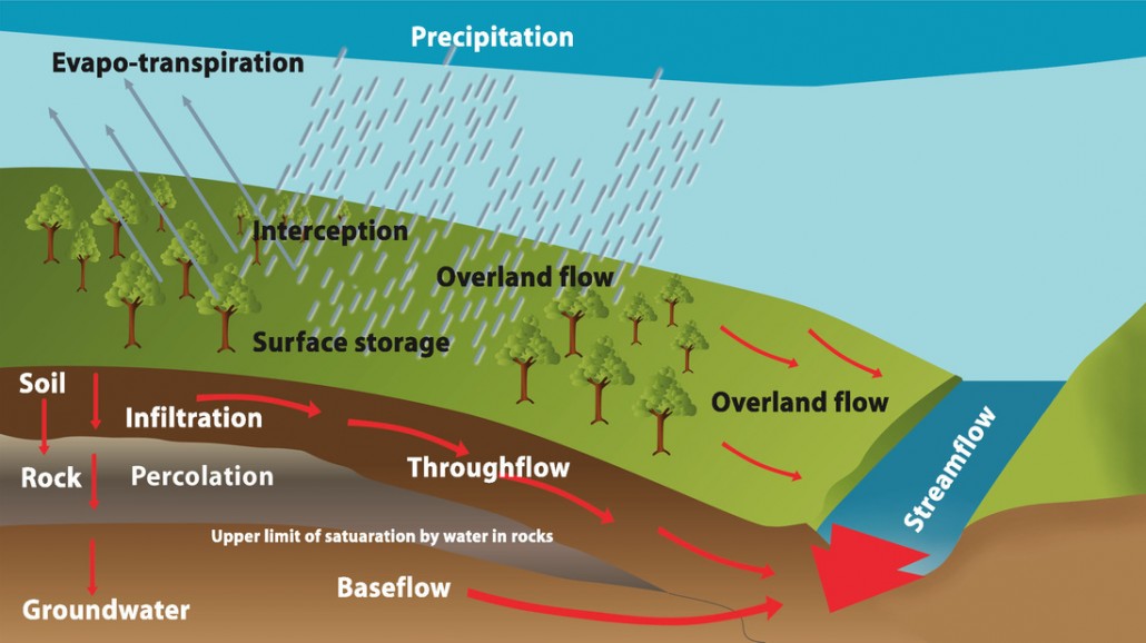
- Any process that results in water moving toward channelized flow, following precipitation reaching the surface.
- Mechanisms responsible for delivering water to streams and rivers.
- River/streamflow: The movement of water in channels toward the ocean.
- Riverflow is typically quantified as discharge: volume of water per unit time
\frac{m^3}{s} .
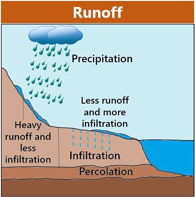 biologyreader.com: Components involved in runoff.
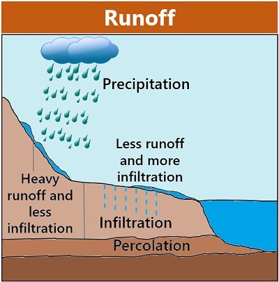
Note the word covers surface flow, water moving downslope within the soil, and groundwater. Most people only picture the first.
Hydrographs and runoff
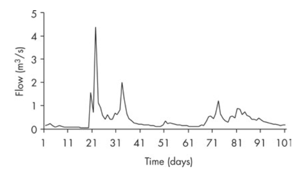
- A continuous record of streamflow is called a hydrograph.
- Peak/storm flow: Water present in a stream during and immediately after a significant rainfall event.
- Globally controlled by rainfall intensity and duration; at catchment scale, affected by catchment size, slope, shape, soil characteristics, vegetation type and cover, degree of urbanisation, and antecedent soil moisture.
- Periods between peaks are referred to as baseflow (distinct from low flow), typically understood to be supplied by groundwater.
“Continuous” is a convenient fiction: a hydrograph is normally an average over an interval, or a sample every 15 minutes.
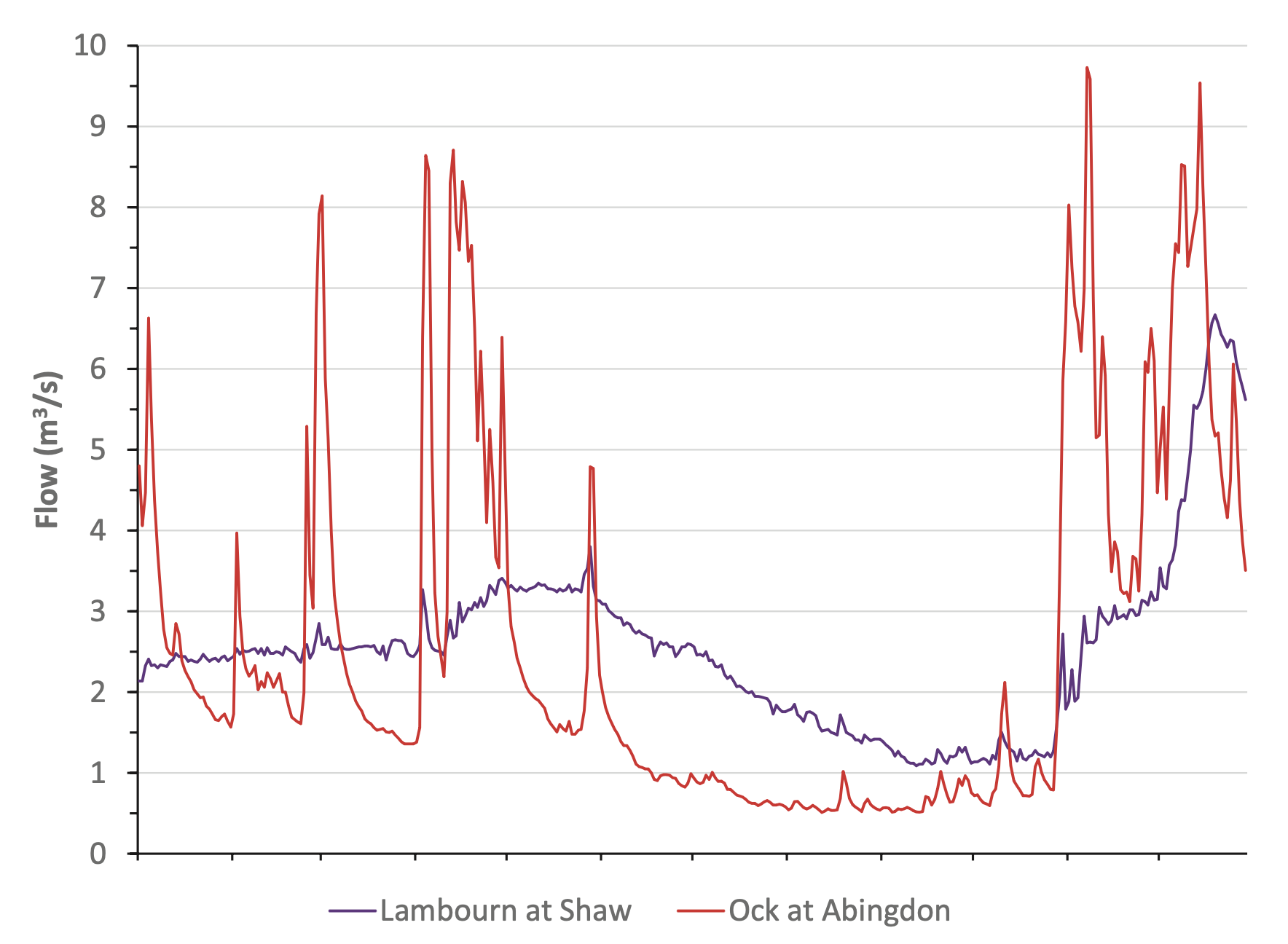
Identical climatic conditions, but different geology. Rocks of the Lambourn are all high permeability, while the Thames catchment is mostly low permeability + bedrock.
Storm hydrograph in detail
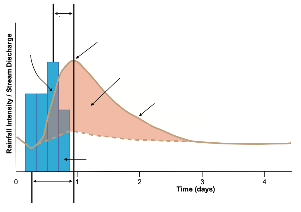
- Rising limb: Steep section leading up to peak flow.
- Contributed by: Channel precipitation (rain falling directly into the stream) and rapid runoff.
- Recession limb: Follows the peak and shows a gradual decline in streamflow.
- Influenced by stormwater arriving from upstream and contributions from subsurface flow.
The exact proportion of precipitation that becomes channelized flow is difficult to determine.
Reading a hydrograph: four measurable quantities
What we take off the curve
- Time to rise: from the start of the rising limb to peak flow.
- Lag time: from the rainfall event to the peak. The single most useful descriptor of catchment response speed.
- Peak flow: the maximum discharge.
- Storm volume (
m^3 ): the area under the curve above the dotted baseflow line.
Each is set by the same physical properties: size, slope, shape, hydraulic length, drainage density, soil, geology, land cover, and antecedent wetness.
A practical point about axes
Hydrographs are often plotted with a logarithmic
On a linear axis, one large event compresses every normal flow onto the
Some texts claim channel precipitation appears as a small blip before the rising limb. In practice this is almost never observed — storm runoff is too messy.
Runoff Mechanism
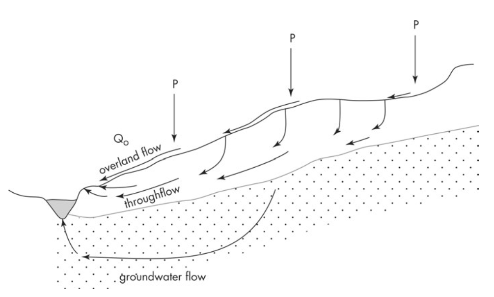
Continuous sheets of overland water flow are rarely observed in nature.
- Overland flow: Water flowing over the land surface after precipitation.
- Horton (1933): Overland flow occurs when rainfall intensity exceeds the infiltration capacity of the soil.
Excess water then flows as a shallow surface layer.
Infiltration capacity acts as a threshold. However, in most cases, infiltration rates exceed typical rainfall intensities.
Runoff Mechanism
Continuous sheets of overland water flow are rarely observed in nature.
- However, in most cases, infiltration rates exceed typical rainfall intensities.
| Soil and vegetation | Infiltration rate (mm/hr) | Rainfall type | Rainfall intensity (mm/hr) |
|---|---|---|---|
| Forested loam | 100–200 | Thunderstorm | 50–100 |
| Loam pasture | 10–70 | Heavy rain | 5–20 |
| Sand | 3–15 | Moderate rain | 0.5–5 |
| Bare clay | 0–4 | Light rain | 0.5 |
Selby (1970) measured 60–600 mm/hour on short grazed pasture in the central North Island of New Zealand. Almost nothing rains that hard.
Runoff Mechanism
- Hursh (1944) coined subsurface stormflow, recognising that flows other than surface flow matter. Cook (1946) proposed that overland flow can also be water that has been underground and re-emerges.
- Betson (1964): Introduced the concept of partial contributing areas — only specific parts of a catchment produce overland flow.
The importance of infiltration is retained, but the idea of uniform thin flow is questioned. - Hewlett & Hibbert (1967): Overland flow occurs when the water table rises to the surface due to infiltration and throughflow.
This results in saturated areas near channels and lower slopes where return flow and direct precipitation dominate. - Confirmed by the field study of Dunne & Black (1970).
Who was right?
Ideas on stormflow
- All theories capture aspects of the truth.
- Saturated overland flow dominates in humid, mid-latitude regions.
- The variable source area concept best represents stormflow processes.
- In arid/semi-arid zones, intense rainfall and low infiltration lead to flash flooding.
- These mechanisms are not exclusive: they can operate in the same catchment at the same time.
| Horton | Betson | Hewlett and Hibbert | |
|---|---|---|---|
| Infiltration | Governs overland flow | Governs overland flow | All rainfall infiltrates initially |
| Overland flow mechanism | Infiltration-excess | Infiltration-excess | Saturated overland flow |
| Contributing area | Uniform across the catchment | Confined to specific zones | Varies in time and space |
Comparison of key theories explaining stormflow generation
A useful framing: Horton asked how fast can water get in?; Hewlett and Hibbert asked is there any room left?
When Horton is right: surfaces that will not take water
Where infiltration excess really happens
- Compacted soils: vehicle wheelings, stock camps, tracks.
- Roads, roofs and paved areas: infiltration essentially zero.
- Crusted soils: a thin surface seal after raindrop impact.
- Hydrophobic soils: repel water on first contact.
Basher & Ross (2001), market gardens in the North Island of New Zealand: infiltration capacity of 400 mm/hour, rising to 900 mm/hour in the growing season — but as low as 0.5 mm/hour in the wheel tracks of the same site.
Hydrophobic soils
Some soils swell rapidly on contact with water and form a temporary impermeable barrier at the surface. Linked to mycorrhizal fungi and to swelling clays such as allophane (Doerr et al. 2007).
Hydrophobicity is temporary. Clothier et al. (2000): a yellow-brown earth/loam went from 2 mm/hour initially to 14 mm/hour once the repellency broke down.
So infiltration capacity is not a fixed soil constant. It varies with land management, with season, and even during a single storm.
Where does a catchment actually saturate?
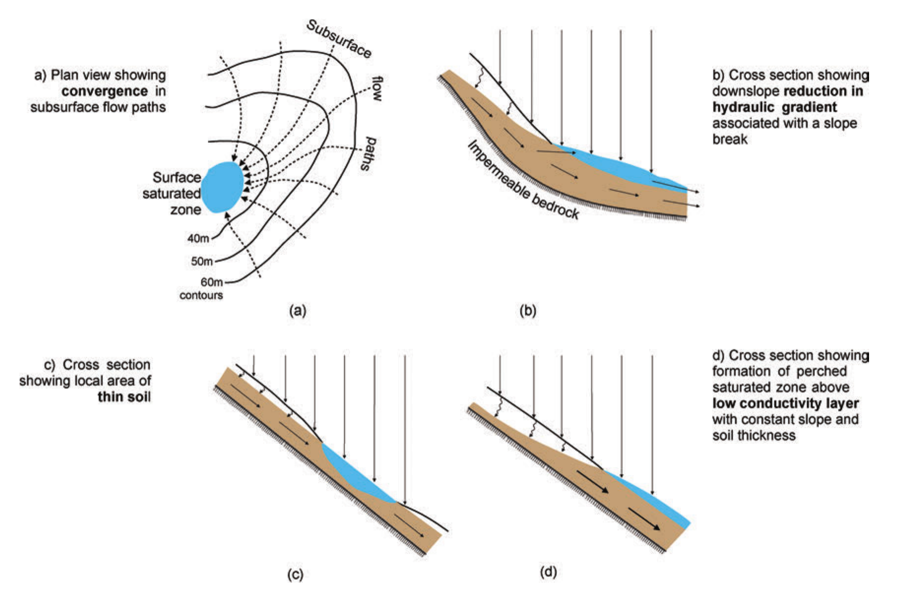
Hewlett and Hibbert placed the saturated areas next to the channel. Later work (Dunne & Black 1970; Anderson & Burt 1978) found four other geometries that force water back to the surface:
- panel a — convergence of subsurface flow into a hillslope hollow,
- panel b — a slope break that reduces the hydraulic gradient,
- panel c — a local thinning of soil over an impermeable base,
- panel d — a drop in hydraulic conductivity, producing a perched saturated zone.
In each case the soil volume receiving the throughflow is too small for the water arriving, so it returns to the surface. This is what the boggy patches at valley heads and slope bases actually are.
These are disjunct source areas: they are not beside the stream. They only add to stormflow if they are hydrologically connected to the valley bottom. Connectivity, not just saturation, controls the hydrograph.
Subsurface flow
- The variable source area model proposes that only parts of the catchment contribute to the hydrograph.
- Overland flow alone can’t explain total discharge observed in hydrographs.
- The gradual decline in the hydrograph’s recession limb suggests a subsurface flow component.
- Tracer studies show significant presence of older water during stormflow.
- This points to throughflow and groundwater contributions.
Throughflow
- Throughflow: Movement of water through the unsaturated zone (soil matrix).
- Described by the Darcy or Richards equations.
- Flow is not only vertical; on slopes, water moves laterally downslope.
- Example: Fine sandy loam → ~13 mm/hour flow rate (Kelliher & Scotter 1992).
The old water problem
The observation that changed the field
Isotope and chemical tracer studies (Martinec et al. 1974; Fritz et al. 1976) show that a large fraction of the water in a storm hydrograph was already in the catchment before the storm started.
The rain that falls during a storm is largely not the water that arrives in the river during that storm.
And yet matrix throughflow is far too slow: 13 mm/hour will not move water down a hillslope inside a storm.
So what does the work?
Three candidate mechanisms, all of which move pressure faster than they move water:
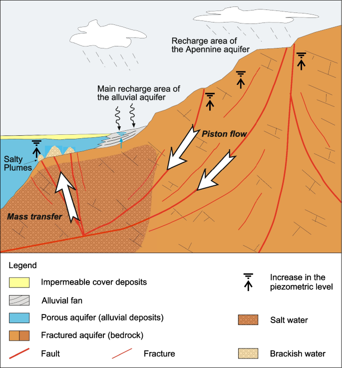
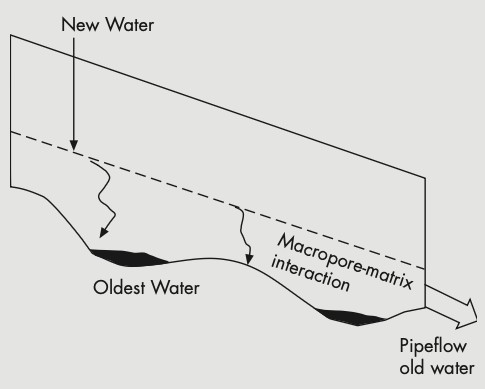
- Piston (translatory) flow — new water at the top displaces old water at the bottom.
- Macropores and pipes — rapid preferential paths through the matrix.
- Groundwater ridging — a rapid saturation response next to the channel.
These are not alternatives to each other. At Maimai all three appear together.
Piston Flow
- Proposed by Horton & Hawkins (1965) — a different Horton from the one behind Hortonian overland flow.
- Water entering at the top of the soil column displaces older water at the bottom, which then enters the stream.
- Similar to a piston where top pressure pushes fluid at the bottom.
- The discharge can be viewed as a pressure wave, so it is modelled as pressure propagation rather than by tracking water particles.
- Though unconventional, the combination of rainfall above and impermeable bedrock below creates this piston effect. Demonstrated in laboratory soil columns by Germann & Beven (1981).
- The added water generates a hydraulic gradient that drives water movement along the base of the soil layer, which typically has higher conductivity (Brammer & McDonnell 1996).
- Analogy: A thatched roof—water moves quickly along aligned channels, especially in the downslope direction (Ward 1984, after Zaslavsky & Sinai 1981).
Macropores
Macropores
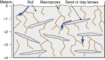
Large, interconnected pores in soil, generally >3 mm in diameter. Formed by cracking, worm burrows and other biotic activity.
- Key pathway for rapid subsurface flow.
- Hydrological role: Enable fast water movement bypassing much of the soil matrix.
- Ongoing debate: Whether these pores form continuous flow networks or are limited by disconnected segments.
- Pipes are the continuous end-member (Jones 1981; Tanaka 1992). Where they exist they dominate hillslope hydrology, but they are not common.
Current view: there is little evidence of macropore networks carrying large volumes continuously to the stream. Their clearest role is delivering water rapidly down to the saturated layer (Heppell et al. 1999), which can then drive piston flow (McGlynn et al. 2002).
Groundwater contribution
- Historically, groundwater was thought to only contribute to baseflow.
- Sklash & Farvolden (1979) introduced the capillary fringe hypothesis to explain the groundwater ridge observed next to streams by Ragan (1968).
- Concept: A “groundwater ridge” forms near the stream during recharge.
- Added infiltration takes soil water next to the channel from tension (unsaturated) to positive pore pressure (saturated), generating hydraulic gradients that drive discharge to the stream.
- The water-saturation relationship in soils is nonlinear, so a small amount of water produces a large change in state.
- This increases both the rate of discharge and the size of the groundwater discharge area.
- Crucially, the ridge develops before any throughflow arrives from upslope.
Ridging has been observed in the field (McDonnell 1990), but it is hard work: instrument response times are often too slow to catch the pore-pressure change.
Case study: Maimai, New Zealand
The site
Established 1974 near Reefton, South Island, to study logging of native beech forest. Short steep slopes (~300 m at ~35°), thick vegetation, incised channels, tiny valley bottoms.
Rainfall ~2,600 mm/yr over ~156 rain days. Stormflow is 65 per cent of total streamflow.
A sequence of results, each overturning the last:
- Mosley (1979, 1982): dye tracing in cut soil faces suggested rainfall could reach the stream in under 3 hours via macropores.
- Pearce et al. (1986): isotopes showed the streamflow was mostly old water — so macropore flow was not the main mechanism.
- McDonnell (1990): groundwater ridging occurs, but there is not enough near-stream water to supply all the old water.
- McGlynn et al. (2002): a combined model — macropores deliver water fast to bedrock, then piston flow along the interface pushes old water out.
How relevant is Maimai?
Maimai has shaped hydrological thinking worldwide. But the conditions are extreme:
- infiltration rates in excess of 1,600 mm/hour,
- soils that stay within 10 per cent of saturation for most of the year,
- short, very steep slopes, very frequent rain.
These conditions are not common, and the concepts do not generalise easily.
The most transferable lesson from Maimai is not a mechanism at all. It is that even under conditions ideal for stormflow generation, the mechanisms remain complex and spatially variable. That is true everywhere.
A summary of different processes
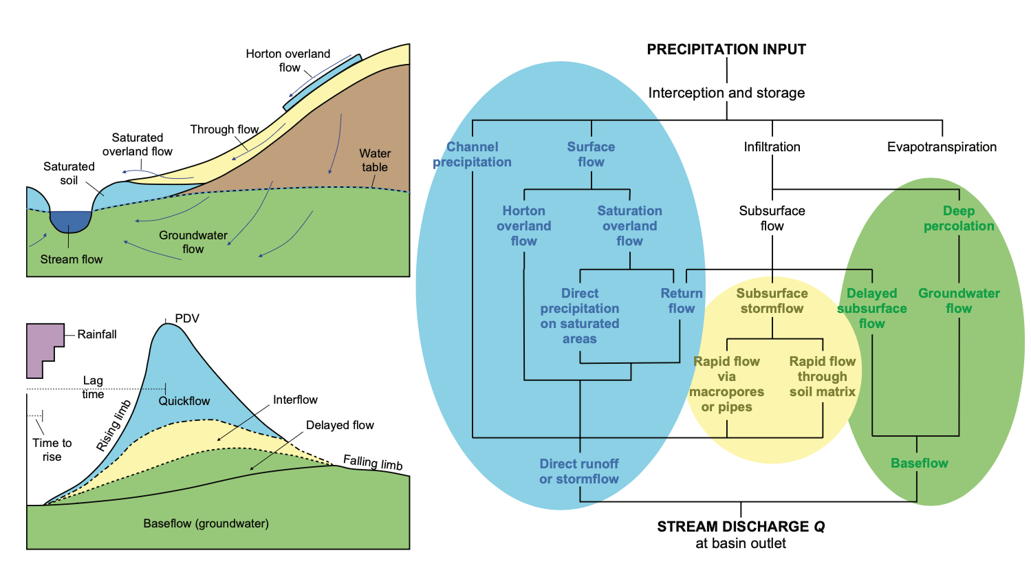
All four mechanisms, one catchment, at once
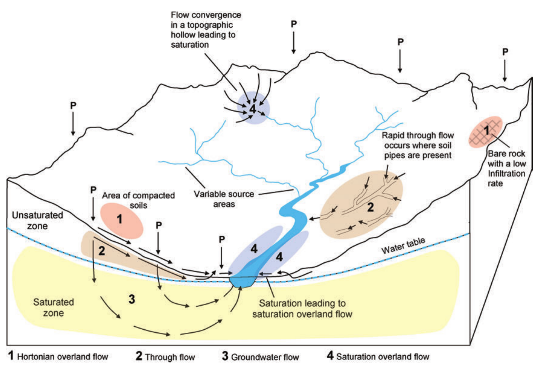
The question is never which mechanism operates. It is which one dominates here, now, and how much of the catchment it covers.
The problem of scale
Hillslope scale (< 10 km²)
Runoff generation mechanisms control the hydrograph. Infiltration capacity, saturation, macropores and piston flow all matter, and they are measurable.
This is the scale of nearly every process study in this lecture, Maimai included.
Large basin scale
The timing of the peak and the shape of the hydrograph are set mostly by the channel drainage network and by the spatial and temporal pattern of the storm.
The hillslope mechanisms are still operating, but they are averaged over so much heterogeneity that they stop being the controlling factor.
This is why a result measured on a 1 km² research catchment cannot simply be scaled up to the Murray—Darling. Keep the scale of a claim attached to the claim.
Baseflow
In sharp contrast to the stormflow debate, there is general consensus here: the major source of baseflow is groundwater, with a smaller contribution from throughflow.
- Water infiltrates, reaches the saturated zone, then moves downslope towards the stream.
- A stream or lake often occurs where the regional water table intersects the surface — though not always.
- Baseflow is usually not visible. Springs are the exception. Most of it is slow seepage through the streambank and bed.
- The only way to detect it is repeated discharge measurement down a reach: if discharge grows with no tributary inflow, the reach is gaining.
Careful with two words
Baseflow is the slow, groundwater-fed component between storm peaks.
Low flow is a statistic of the flow record — how small the discharge gets in a dry period.
They are related but they are not the same quantity, and they are analysed with different tools.
Channel flow
Once water reaches the stream, the rate of flow depends on three things:
- the volume of water present,
- the gradient of the channel,
- the resistance at the channel bed.
This is described by uniform flow formulae — Chézy and, more commonly, Manning:
with
Remember this equation. We will meet it again when a satellite tries to estimate discharge without ever touching the river.
Ephemeral channels
In arid regions many channels flow only during floods. The resistance problem there is complicated by infiltration through the bed.
The first flush of water fills the available pore space in the bed, so it:
- loses volume from the stream, and
- slows the flood front as it advances over a rough, dry surface.
These transmission losses are why an arid-zone flood peak can shrink dramatically as it travels downstream.
Measuring hillslope runoff
There is no standard method
Overland flow: runoff plots
A runoff plot is a bounded area of hillslope. Metal plates are driven into the soil along the upslope and side boundaries and left protruding, so every drop of overland flow generated inside the plot is captured.
The collected flow is routed to a tipping bucket or a temporary flume and recorded as volume per unit time.
- Overland flow varies enormously in space and time, so several plots are needed to characterise one slope.
- A rainfall simulator can be used to impose a controlled, repeatable input instead of waiting for a storm.
Throughflow: troughs and tracers
To measure throughflow you must dig a trench perpendicular to the flow direction and insert troughs at the depths of interest, then backfill.
The act of measuring changes what you measure. Digging disturbs the profile, and the loosely reconstituted soil in front of the troughs is a preferential path, so throughflow is often overestimated.
Alternative: subsurface tracing with a conservative tracer that does not bind to soil — sodium chloride, bromide, or fluorescent dyes such as Rhodamine WT.
This is the honest reason our understanding of runoff mechanisms is still incomplete. The measurements are hard, disturbing, and site-specific.
Measuring streamflow
Velocity-area method
- The velocity–area method multiplies stream velocity by cross-sectional area to estimate discharge.
- Black dots: locations of velocity readings.
- Dashed lines: triangular/trapezoidal cross sections.
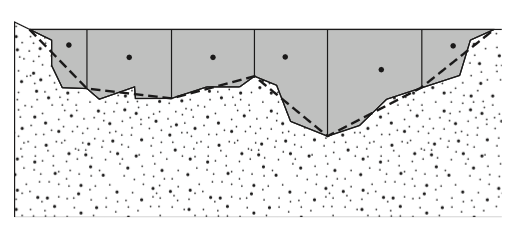 The velocity–area method of streamflow measurement. The black circles indicate the position of current meter velocity readings. Dashed lines represent the triangular or trapezoidal cross-sectional area through which the velocity is measured.
Velocity–area method: considerations
The velocity–area method requires the assumption that the velocity measured is representative of the entire cross-sectional flow.
Since multiple measurements across the depth are rarely feasible, adjustments are needed to account for velocity variations.
Water flows faster near the surface than near the bed due to bed friction.
A general guideline: measure velocity at 60% of depth from the surface (or 40% above the bed).
For deeper rivers, average readings at 20% and 80% of depth for better accuracy.
If no velocity meter is available, a float method can provide rough estimates by timing surface travel over a measured distance.
Surface floats overestimate true velocity since they ride faster-flowing surface water.
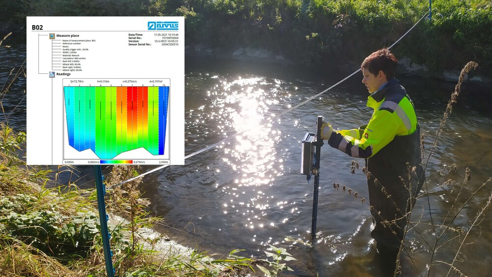
- The velocity–area method works well for small rivers, but its accuracy depends on sampling strategy.
- It becomes less reliable in turbid, shallow, or rough-bedded streams (e.g., mountain creeks).
- In such cases, consider alternative methods like dilution gauging. Illustration of float-based surface velocity measurement
Stage–Discharge Relationship
Stage = water level or height at a specific point in a river.
Discharge = volumetric flow rate (e.g.
\frac{m^3}{s} ).Repeated discharge measurements (via velocity–area method) enable creation of a rating curve.
A rating curve relates stage to discharge and allows continuous discharge estimation from simple stage measurements.
Developed by pairing stage readings (e.g. using a stilling well) with discharge data.
Rating curves are typically non-linear, reflecting the geometry of riverbanks:
As rivers fill between banks, more water is required to raise stage than at low flows.Assumes a stable riverbed. Changes (e.g. due to flood scouring or deposition) will invalidate the curve.
This is why flumes or weirs are often installed to stabilize the control section.
Limitations:
- Few high-flow measurements → less reliable for peak floods.
- High-flow events are dangerous and infrequent.
- Thus, errors increase at the upper end of the curve.
Remember: discharge is inferred from measured stage — not directly observed. 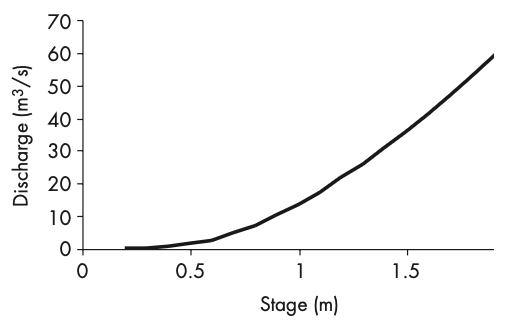
Flumes and weirs
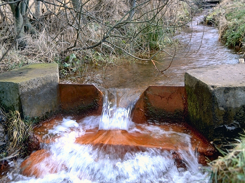
- In principle the same as stage-discharge relationship, but with a control section.
- Flumes and weirs are stream gauging structures that extend the stage–discharge method by imposing control over stream velocity and cross-sectional area.
- By doing so, they provide a continuous record of stream discharge.
- The key is to standardize flow through a known cross-sectional area so that velocity becomes predictable or known.
- This is especially useful because stream velocity varies with depth, but gauging structures enforce a consistent flow regime.
- These structures are designed so that discharge becomes a function of stage alone.
Discharge equations for weirs
- Discharge through weirs is determined by known formulas based on weir shape.
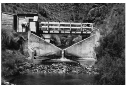
- For a V-notch weir (Very accurate for low-flow rates):
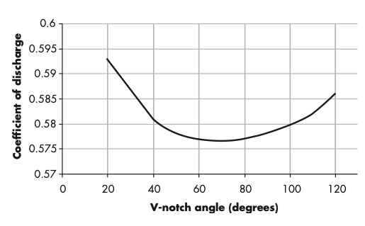
Q = 0.53 \sqrt{2g} \, C \, \tan\left(\frac{\theta}{2}\right) b^{2.5} - Where:
Q = discharge (\text{m}^3/\text{s} )g = gravity (9.81\text{m}/\text{s}^2 )C = discharge coefficient (depends on\theta )\theta = notch angleb = stage height (m)
- For a 90° V-notch,
C = 0.578 , and:Q = 1.366\ b^{2.5} - These equations follow ISO 1438 standards for gauging structures.
Flumes and weirs: design considerations
- The shape of the gauging structure affects sensitivity to changes in flow:
- V-notches are excellent for low flows due to higher sensitivity.
- As discharge increases, cross-sectional area expands nonlinearly.
- Under high flows, it’s crucial that water doesn’t bypass the structure.
- V-notches are commonly used with 90° or 120° angles based on application needs.
- Stilling ponds slow down water before measurement but can trap sediment.
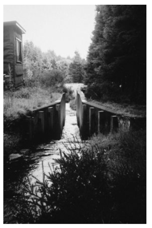
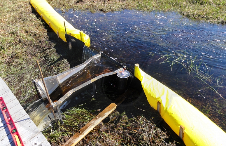 A trapezoidal flume helps flush sediment
Flumes vs. weirs
- Flumes and weirs both allow continuous measurement of stream discharge but have key differences:
- Weir: Water flows over a structure (like a small waterfall).
- Flume: Water flows through a structure without dropping.
- Flumes tend to produce less sedimentation, making them suitable for high-energy environments.
- Trapezoidal flumes can flush out sediment efficiently, avoiding stilling pond build-up.
- Both are suitable for small streams but not large rivers, due to structural stress.
Streamflow from space
Why we want a river gauge in orbit
Everything on the last few slides needs a person to stand in, or beside, a river.
- The global gauge network is shrinking, and many national records are not shared.
- Whole basins in Africa, central Asia and South America have no publicly available discharge record.
- The measurements we most want — the flood peaks — are the ones that are dangerous to make and that destroy the gauge. In Mozambique in 2000, most gauges were inundated or washed away, so the return period of the flood could not be established afterwards.
The awkward fact
A satellite cannot measure discharge.
Discharge is a volume flux through a cross-section. Nothing in a reflected radar pulse carries velocity or bed geometry.
What a satellite can see is:
- water surface extent — where the water is,
- water surface elevation — how high it is,
- and, if it sees enough of the reach, the water surface slope.
Which is exactly the position a hydrologist is in at a stilling well. We measure stage and infer discharge. Space-based hydrology plays the same trick from 890 km up.
Nadir altimetry: virtual gauges
A radar altimeter sends a pulse straight down and times the return. Range plus precise orbit determination gives the height of the surface above a reference ellipsoid.
- Designed for the ocean: TOPEX/Poseidon (1992), the Jason series, Sentinel-3, Sentinel-6 Michael Freilich, CryoSat-2.
- Repurposed over land. Where a ground track crosses a river, we get a time series of water height: a virtual station.
- Repeat cycles: ~10 days (Jason, Sentinel-6), ~27 days (Sentinel-3).
What nadir altimetry cannot do
- The tracks are fixed. Most rivers are never crossed, and the crossing is rarely where you want a gauge.
- The footprint is kilometres across, so the return from a narrow river is contaminated by the banks and the floodplain.
- You get a height at a point, not a slope along a reach, so the flow gradient is unknown.
A single height, at a place we did not choose, every 10 to 27 days. Useful for the Amazon. Not useful for most rivers.
SWOT: from a line to a swath
Surface Water and Ocean Topography — NASA and CNES, with CSA and UKSA. Launched 16 December 2022.
The instrument is KaRIn, a Ka-band radar interferometer: two antennas on a 10 m boom. The phase difference between the two returns gives the height of every pixel, so it maps elevation over an area rather than along a line.
- Two 50 km swaths either side of a 20 km nadir gap: 120 km total.
- Pixels roughly 10–70 m across track, ~20 m along track.
- 21-day repeat, with 2–4 looks per cycle at mid latitudes.
- Requirement: rivers wider than 100 m (goal 50 m); lakes larger than about 250 m × 250 m.
Why the swath matters
For the first time we obtain, for the same reach and the same overpass:
- the width
W of the water surface, - the water surface elevation,
- and the slope
S along the reach.
Slope is the quantity nadir altimetry could never give, and it is the one that Manning’s equation demands.
Products are reported on ~10 km reaches defined in the SWORD river database.
From height and slope to discharge
Recall the uniform flow law from the channel flow slide:
SWOT supplies
It does not supply:
- Manning’s
n , the roughness, and A_0 , the unobserved cross-sectional area beneath the lowest water surface ever seen.
Both must be estimated from many repeat passes, from prior information, or from a model.
The same caution, one more time
On the rating curve slide we said: discharge is inferred from measured stage, not directly observed.
Nothing about being in orbit changes that. A SWOT discharge value is the output of an inversion with two unknowns, constrained by observations of the water surface.
So ask of any satellite discharge product exactly what you would ask of a rating curve: how many observations constrain it, over what range of flows, and how far is this estimate extrapolated beyond them?
What space does not fix
Hard limits
- No velocity. Roughness and geometry stay unknown; they are inferred, never measured.
- Width threshold. Channels narrower than about 50–100 m are invisible, and most of the world’s channel length is narrow headwater stream.
- Sampling. A 21-day repeat can miss a flood peak completely — and flood peaks are what we most want.
- Interference. Overhanging vegetation, ice, and very flat water surfaces all degrade the retrieval.
What it changes anyway
- Reach-scale water surface elevation and slope for large rivers worldwide, including basins with no gauge and no data-sharing agreement.
- Lake and reservoir storage change, which closes the other half of the surface water budget.
- A consistent measurement, made the same way everywhere, against which national records can be compared.
The right way to think about SWOT is not as a replacement for gauges. It is a global, uniform, sparse-in-time observation that is most valuable exactly where the ground network is thinnest.
Floods
What is a flood?
A working definition: inundation of land adjacent to a river, caused by a period of abnormally large discharge.
Every word of that is negotiable.
- Flooding also comes from the sea and from lakes.
- “Abnormal” depends entirely on the length of record you happen to hold.
- Floods reach our attention through damage, so they are usually rated in dollars, not in cumecs.
As with rainfall, the frequency–magnitude relationship governs: small floods are common, the large ones are rare and do nearly all the damage.
Hydrological size and human cost are different quantities
China, 1998 — ~US$20 billion damage, 15 million people displaced, 3,000 lives lost.
Mississippi and Missouri, 1993 — US$15–20 billion, 48 lives lost. Hydrologically the far larger event: the highest in the record, with an average recurrence interval of 100–500 years.
Similar cost. A factor of sixty in lives. The difference is not hydrology, it is warning, infrastructure and wealth.
What makes a flood bigger — part 1
Antecedent soil moisture
The largest influence on flood size after the rainfall itself.
Infiltration, and therefore storm runoff, depends on how saturated the soil already is. Almost every major flood is preceded by a wet period.
Deforestation
Forest reduces flood severity through three mechanisms we have already met: interception, high organic matter in the upper soil, and higher infiltration rates.
Fahey & Jackson (1997): converting tussock grassland to pine plantation reduced mean flood peaks by 55–65 per cent — in a small New Zealand research catchment.
Urbanisation
Impervious surfaces generate infiltration-excess overland flow, and the drainage system is deliberately engineered to remove it fast, straight into the river network.
Cherkauer (1975) found a large increase in flood magnitude for an urban catchment in Wisconsin compared with a similar rural one.
A recurring caveat
Each of these effects is measured convincingly at the small catchment scale (< 10 km²).
At the whole-basin scale the urban fraction is small, the forest change is patchy, and the signal becomes very hard to detect. The same problem of scale, again.
What makes a flood bigger — part 2
Channelisation
A natural channel is broadly in equilibrium with the flows it carries. Rigid engineering breaks that adjustment.
Channelisation is usually built to reduce flood risk locally — and usually succeeds. But it passes water downstream faster than before, increasing the risk downstream. If there is a floodplain down there, no harm. If there are people, harm.
Land drainage
Draining “swamp” land for agriculture makes the land drier, so small events produce less runoff.
But rapid removal through drains and ditches means that when a large event comes, the water reaches the channel network far faster than it naturally would. Drier land, sharper peaks.
Climate change
Every flood now prompts an immediate question about climate. It is a hard question, because climate is naturally very variable and single events are weak evidence.
What can be said:
- projections consistently indicate more high-intensity rainfall events,
- channel geometry adjusts slowly to a changed flow regime,
- so risk is elevated during the adjustment period — if the channel is allowed to adjust at all.
Attribution of a single flood to climate change is a statistical exercise on the rainfall, not a hydrological statement about the flood. Keep the two separate.
Case study: Mozambique, 2000
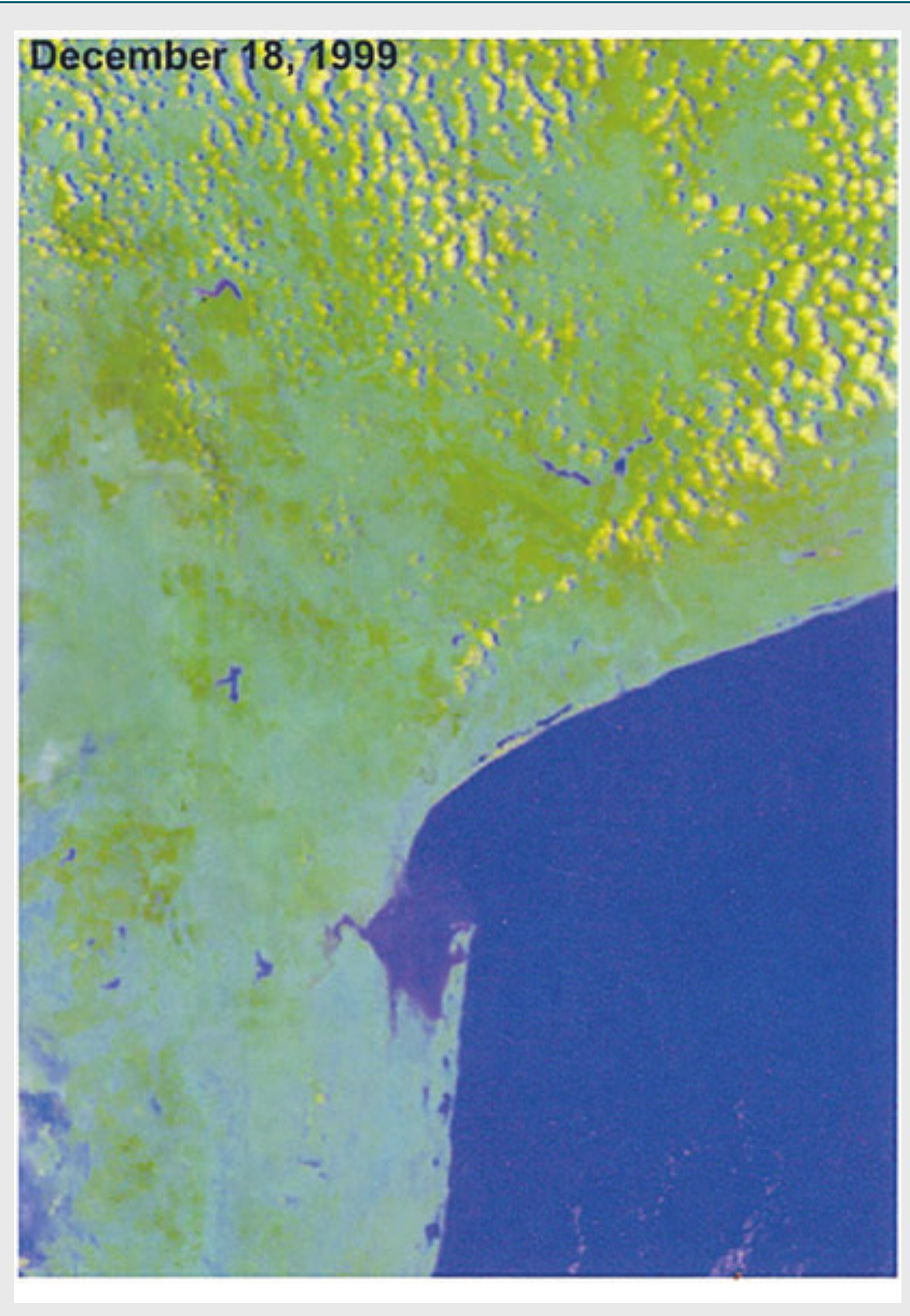 18 December 1999
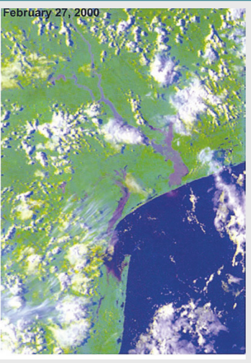 27 February 2000
- Four floods in succession, January to March 2000.
- Preconditioning: rainfall at Maputo was 70 per cent above normal in October–November 1999, so the catchments were already saturated.
- Cyclones Connie, Eline and Glória each delivered record rainfall inland over Zimbabwe and northern South Africa.
- The Limpopo rose 3 m higher than any recorded flood. For the first time in the record, the Limpopo and Incomáti joined into a single inundation.
- 700 people died; 45,000 were displaced; ~US$450 million of infrastructure damage.
- Flood warnings were issued upstream by Zimbabwe and South Africa. Communications inside Mozambique had already been cut by the earlier floods.
Most gauges failed, so the return period was never established. The satellite images are the record.
Images courtesy of G. Robert Brakenridge, NASA-supported Dartmouth Flood Observatory.
Case study: Brisbane, 2010–11
- Brisbane River catchment, 13,570 km²; mostly grazing and forestry, but Brisbane (1.98 million) and Ipswich (200,000) sit in the lower reaches.
- A strong La Niña, with very warm sea surface temperatures off the Queensland coast, drove exceptional rainfall from late November 2010.
- Six large rainfall events made December 2010 the wettest December on record for southern Queensland. The soil was fully saturated.
- Rainfall for 10–12 January 2011 had an annual exceedance probability of 1 in 150 over the catchment, exceeding 1 in 500 in places.
- Peak in Brisbane City: 13 January 2011. Seventh highest river height since records began in 1840, highest since 1974.
- 37 people killed, 29,000 homes and businesses inundated, ~A$5 billion in insurance and recovery.
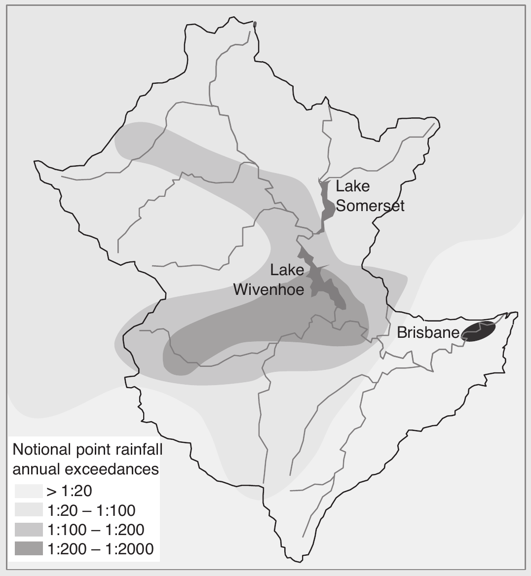
Brisbane 2011: what the numbers actually show
Antecedent moisture did the work
Catchment-average rainfall, 10–12 January 2011: 286 mm.
Catchment-average rainfall, 25–27 January 1974: 349 mm.
Less rain in 2011 — yet nearly double the flood volume of 1974, and the highest inflows on record above Wivenhoe Dam.
The difference is the saturated December soil. This is the antecedent soil moisture control, at basin scale, in a single comparison.
The dam
Wivenhoe (1958) and Somerset (1985) exist primarily for water supply; Wivenhoe also provides flood mitigation.
By 7 January both were above full storage and were releasing. By 11 January they had recovered enough storage to pass only 60 per cent of inflows, holding back 40 per cent.
Estimated effect: the Brisbane peak was reduced by about 2 m, and ~14,000 properties were spared.
The Queensland Commission of Inquiry concluded the dam operations achieved the best possible flood mitigation effect.
The dam operator’s real problem: hold back as much water as possible, while keeping enough empty storage for rain that has not fallen yet. The decision depends entirely on a rainfall forecast — the least predictable quantity in the whole system.
Brisbane 2011: why everyone blamed the dam
Despite the Inquiry’s finding, the public narrative fixed on Wivenhoe. Four reasons, and none of them hydrological:
- The summer of 2010–11 followed an extreme drought. A year earlier there were serious concerns Brisbane would run out of potable water, so the prevailing story was of empty dams.
- There had been no major flood since 1974, so flooding was outside the collective memory of most residents.
- Wivenhoe was built after 1974, which created a sense of security that flooding had been solved.
- Modern societies want an immediate scapegoat for a natural disaster.
Nathan (2012): lessons from large floods
- Big rains cause big floods.
- Communicating risk is difficult.
- Hydrologic complexity cannot be ignored.
Deceptively simple, and worth pinning to a wall. Note that two of the three are not about hydrology at all.
Infrastructure lowers the frequency of flooding. It does not remove the hazard, and it reliably raises the exposure behind it.
Mapping floods from space
Two ways to see water from orbit
Optical: Landsat, Sentinel-2, MODIS
Water absorbs strongly in the near-infrared and shortwave infrared, so it is dark in those bands while vegetation and soil are bright.
Band ratios such as NDWI and MNDWI exploit exactly that contrast to separate water from land.
- Long archive (Landsat since the 1980s), familiar, easy to interpret.
- Fatal weakness: cloud. Floods arrive with the weather that caused them, so the optical sensor is blind at the moment of peak inundation. The Mozambique image of 27 February 2000 is patchy with cloud for this reason.
Radar: Sentinel-1 C-band SAR
Calm open water is a specular reflector: it bounces the radar pulse away from the sensor, so it returns almost nothing and appears very dark.
Radar supplies its own illumination and penetrates cloud, so it works at night and through the storm.
- False positives: smooth dry surfaces — tarmac, dry sand, salt pans — also look dark.
- False negatives: wind-roughened water scatters back and looks like land; flooded vegetation can look bright through double-bounce off trunks and the water surface.
Neither sensor sees depth. Extent plus a digital elevation model gives an estimate of depth and volume — with all the error of the DEM folded in.
From single images to a flood record
Dartmouth Flood Observatory
The source of the Mozambique images in the textbook. A global, near-real-time flood catalogue built from satellite imagery, running since 1985.
It exists because for most of the world’s floods, satellite imagery is the only consistent record — the gauges are missing, or drowned.
Digital Earth Australia — Water Observations from Space
Every Landsat observation over Australia since 1987, classified pixel by pixel as water or not-water at 25 m resolution.
You can then ask a question no gauge can answer: how often has this pixel been wet?
What that buys you
- A flood frequency map built from observation rather than modelling.
- Wetland and floodplain inundation history for ecological water requirements — central to Murray—Darling Basin planning.
- Detection of where floodplains have been disconnected from their rivers by levees and development.
Notice the pattern across this whole lecture. Ground methods measure the right quantity at one point. Satellite methods measure a proxy everywhere. Hydrology is the work of joining the two.
Runoff and water quality
The route water takes from raindrop to river largely determines its chemistry, because chemistry is set by contact time with the soil.
- Water arriving as overland flow has had little soil contact: low nutrient load, but often high suspended solids picked up from the surface. It looks dirty and is chemically clean.
- Water arriving as throughflow or groundwater has had long contact: higher nutrient load, but clear. It looks clean and is chemically loaded.
So “clear water” and “clean water” are not the same claim.
A consequence of piston flow
When groundwater responds to rainfall, it frequently responds as a pressure wave. The water that enters the stream is not the water that just infiltrated.
That water may be years or decades old, and therefore unaffected by any recent land-use change.
This is why a catchment can be replanted, or a fertiliser regime changed, and the stream chemistry not respond for years. The lag is real, and it is a genuine problem for water policy.
Summary
So here we covered that:
- Runoff is the movement of water toward channels — over the surface, through the soil, and as groundwater — influenced by rainfall, soil, vegetation, and terrain.
- A hydrograph’s lag time, peak and storm volume encode the physical properties of the catchment above it.
- Horton, Betson, and Hewlett & Hibbert offer complementary theories; the variable source area concept, extended by disjunct source areas and connectivity, is the working picture.
- Storm hydrographs are full of old water, delivered by piston flow, macropores, and groundwater ridging rather than by moving new rain quickly.
- Which mechanism matters is a question of scale: hillslope processes control small catchments, the drainage network controls large ones.
- Streamflow is measured on the ground by velocity–area, stage–discharge curves, and gauging structures — and from orbit by altimetry and SWOT, which observe stage, width and slope and still infer discharge.
- Flood magnitude is driven by rainfall and antecedent soil moisture, and modified by deforestation, urbanisation, channelisation and drainage.
- Satellite optical and radar imagery map flood extent where gauges have failed, but they see extent, not depth and not discharge.