- / -
Tutorials
Water Cycle
Water Cycle
Reference: Davie & Quinn (2019), Fundamentals of Hydrology, 3rd ed., Chapter 1.
Almost everything in this course rests on one idea, which is that water is conserved. The lecture stated that idea; this tutorial is where we find out what it is good for. Bring a calculator, and work in small groups so that you can compare answers as you go.
Two of the questions ask you to check numbers that appear in a published textbook. In both cases the number does not come out as printed. This is deliberate, and it is not a trap. Textbooks are written by people under deadline, figures are redrawn by third parties, and units get lost in the retyping. Getting a different answer from the book is a sign that you have done the arithmetic, not that you have made a mistake, and learning to trust a calculation you have done yourself over a number you have read is most of what separates a hydrologist from a person who quotes hydrology.
1. The hydrological cycle across scales
Before we compute anything, it is worth being clear about what we are computing.
Define the hydrological cycle and explain how it operates at both the global and the catchment scale. In your answer, describe three key processes and how they interact across the two scales.
The textbook is careful to describe the cycle as a conceptual model containing “gross simplifications”. Name two simplifications that the global diagram makes, and say for each whether it would matter to a hydrologist working on a single catchment.
2. Does the global water cycle balance?
A figure in a textbook is an argument, and arguments can be checked. The global cycle diagram (Davie & Quinn, Figure 1.7) makes a strong claim about how much water moves where, and it gives us enough numbers to test whether that claim is internally consistent.
| Flux | Value (km³/yr) |
|---|---|
| Precipitation over the ocean | 458,000 |
| Evaporation from the ocean | 502,800 |
| Precipitation over the land | 110,000 |
| Evapotranspiration from the land | 65,200 |
| Precipitation over internally draining land | 9,000 |
| Evaporation from internally draining land | 9,000 |
| River run-off to the ocean | 42,600 |
| Groundwater flow to the ocean | 2,200 |
- Work out the net loss from the ocean, being evaporation minus precipitation, and the net gain over the land, being precipitation minus evapotranspiration. What do you notice?
- Now find the total return flow from land to ocean. Does the budget close? If it does, explain in one sentence why it had to.
- Compare global precipitation with global evaporation, and comment on the result.
- Express the 110,000 km³/yr of land precipitation as a mean depth in mm/yr. Which area belongs in the denominator: the
119 \times 10^6 km² that drains to the ocean, or the whole149 \times 10^6 km² of land? Work out both, then decide which one honestly answers “mean precipitation over land”. What would you compare your answer against to check it? - The same figure labels the area of internal runoff as 119 million km² and the area of external runoff as 119 million km², with the oceans at 361 million km². Add the three areas together. The Earth’s total surface area is
510 \times 10^6 km². Something has gone wrong. Which of the three labels do you trust least, and why? Does the error affect your answers to parts 1 to 3, and how do you know?
3. How long does water stay put?
Every drop of rain that has ever fallen passed through the atmosphere, and yet the atmosphere holds less than a thousandth of a percent of the Earth’s water. Those two statements are both true, and reconciling them requires a quantity we have not used yet.
| Store | Volume ( |
|---|---|
| Oceans and seas | 1,338,000 |
| Ice caps and glaciers | 24,064 |
| Groundwater | 23,400 |
| Lakes | 176 |
| Atmosphere | 12.9 |
| Rivers | 2.12 |
| Total | 1,385,984 |
The mean residence time of a store is
where
- Using the fluxes from Question 2, estimate
\tau for the atmosphere, for rivers, for the oceans, and for groundwater. Give each answer in whatever unit makes it readable, whether days, years or thousands of years. - Return to the two statements above and reconcile them using your answers.
- Try to compute a residence time for ice caps and glaciers. Something stops you. What is it, and what would you need in order to proceed?
- Two catchments suffer the same chemical spill, one into a river and one into an aquifer. Using residence times, explain why these are not the same problem, and why the second is worse.
- A store that is part of a cycle is, by definition, replenished. Explain why a store with a long residence time is nevertheless non-renewable in any sense that matters to us.
4. A number worth checking
Davie & Quinn observe that if we count only groundwater within the first kilometre of the surface and set aside snow and ice, roughly 0.27% of the Earth’s water is available for human consumption. They then convert that share into a figure that is meant to reassure, namely about 146 million litres of fresh water per person, for a world population of seven billion. The implication is that scarcity is a distribution problem rather than a supply problem.
Let us see whether the number survives contact with a calculator.
- Reproduce the calculation. Take 0.27% of the total volume in Question 3, convert to litres (
1 km³= 10^{12} L), and divide by7 \times 10^9 people. - Your answer will not be 146 million. By what factor do the two disagree? Working backwards, what volume would give 146 million litres per person, and what percentage of the total is that?
- The textbook attaches the units “per person per day” on p. 8, and “per person per year” on pp. 10 and 11. Both cannot be right. Consider whether either can be, by asking what kind of quantity 0.27% of a store actually is. This is the more important half of the question.
- Now build an honest figure. Global river run-off is 42,600 km³/yr, and it is renewed every year. Share it among eight billion people to get cubic metres per person per year, and compare.
- Place your answer to part 4 in the table below. Does it fall where you would expect a global average to fall? Then explain why the 146 million litre figure could never be compared with this table, even after the units were repaired.
| Country | Renewable water ( | Country | Renewable water ( |
|---|---|---|---|
| Iceland | 525.074 | Kuwait | 0.000 |
| Canada | 81.071 | Egypt | 0.022 |
| Australia | 21.272 | Israel | 0.093 |
| USA | 8.914 | Kenya | 0.467 |
| United Kingdom | 2.262 | South Africa | 0.843 |
5. A year in the life of an inland catchment
We now leave the globe and work at the scale where hydrologists actually earn a living. The data below are synthetic, but the pattern they contain is an ordinary one for an inland catchment in western New South Wales, and part of your task is to work out what kind of year this was.
A catchment of area
| Month | ||||
|---|---|---|---|---|
| Jul | 55 | 4 | +18 | ? |
| Aug | 52 | 5 | +14 | ? |
| Sep | 45 | 5 | +2 | ? |
| Oct | 42 | 4 | -12 | ? |
| Nov | 38 | 3 | -22 | ? |
| Dec | 30 | 2 | -34 | ? |
| Jan | 28 | 1 | -38 | ? |
| Feb | 30 | 1 | -33 | ? |
| Mar | 33 | 1 | -22 | ? |
| Apr | 38 | 2 | -8 | ? |
| May | 50 | 3 | +12 | ? |
| Jun | 59 | 4 | +23 | ? |
- Rearrange the water balance equation to give
E , then compute evaporation for January, April and July, showing your working. Pay attention to what happens to the sign when storage falls. - Complete the annual totals for
P ,Q ,\Delta S andE . - You will find that annual
E exceeds annualP . Before deciding this is an error, ask whether it is physically possible. Explain what the catchment did over the year, where the extra water came from, and whether it could do the same thing again next year. - Compute the run-off coefficient
Q/P . In a humid temperate catchment roughly one third of precipitation becomes surface run-off. Account for the difference. - A depth in millimetres becomes a volume once multiplied by the catchment area,
V = d \times A , and this conversion is worth doing slowly the first time. Express the annual run-off as a volume in m³ and in gigalitres (1 GL= 10^6 m³), and as a mean discharge in m³/s. - Express the storage loss in gigalitres. If a substantial part of that water was groundwater, use the residence time you found in Question 3 to say what “recovery” would actually mean here, and over what timescale.
6. Magnitude, frequency and duration
Two figures from the River Boyd in the United Kingdom appear below. Between them they contain most of what an engineer needs in order to decide how large to build something, and most of the ways in which that decision goes wrong.
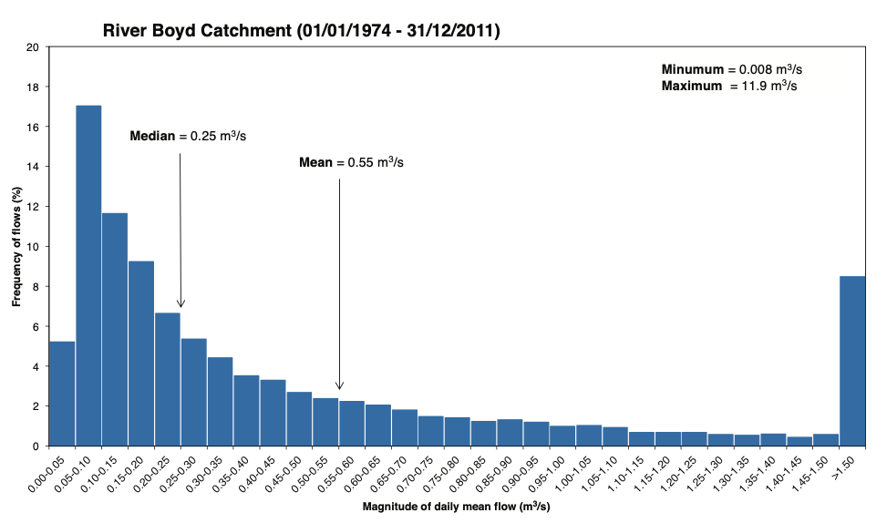
Part A. The flow record. The record covers 38 years of daily mean flows. The median is 0.25 m³/s, the mean is 0.55 m³/s, and the maximum is 11.9 m³/s.
- The mean is more than double the median. Explain why, what that implies about the shape of the distribution, and how it differs from a normal distribution.
- Flows above 9 m³/s occurred on seven days of the record. Use
p = n/N to find the probability of exceeding 9 m³/s on any given day, and express it as a percentage. - Somebody asks you for “the typical flow of the River Boyd”. Which statistic do you give them, and why? Which would you use to size a bridge?
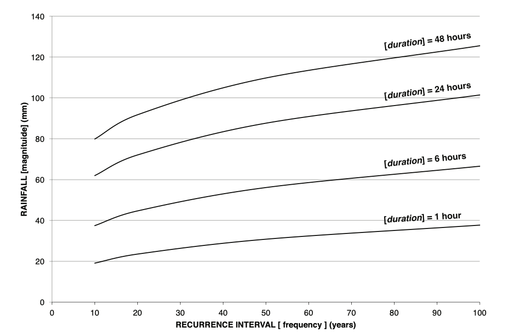
Part B. The design rainfall curves. From the magnitude, frequency and duration curves, read off the rainfall depth for a 20-year recurrence interval at each of the four durations of 1, 6, 24 and 48 hours. Reading a value off a graph is a legitimate hydrological skill, so do not worry about the last millimetre.
- Tabulate depth against duration, then convert each to a mean intensity in mm/h.
- Depth rises with duration while intensity falls. Both trends have physical causes. Give them.
- Which duration would you use to design an urban stormwater drain, and which to design a flood levee on a large river? Justify each choice, and state the general principle that connects them.
Part C. Recurrence intervals.
- A town experienced its “one in a hundred year flood” last year, and a resident argues that the town is therefore safe for some time to come. Using
p = 1/T , explain what is wrong with the reasoning. - Find the probability of experiencing at least one such flood during a thirty-year mortgage. It is easier to compute the probability of experiencing none. Does the answer surprise you?
- Hydrologists prefer the term recurrence interval to return period. Having answered part 7, explain why.
7. Delineating a catchment boundary
There is a standard five-step procedure for this, and you could find it online in about thirty seconds. We would like you to resist, because the procedure follows from two facts you already know, and deriving it will teach you more than memorising it. The map below shows contour lines, a stream in the valley, and a marked outlet.
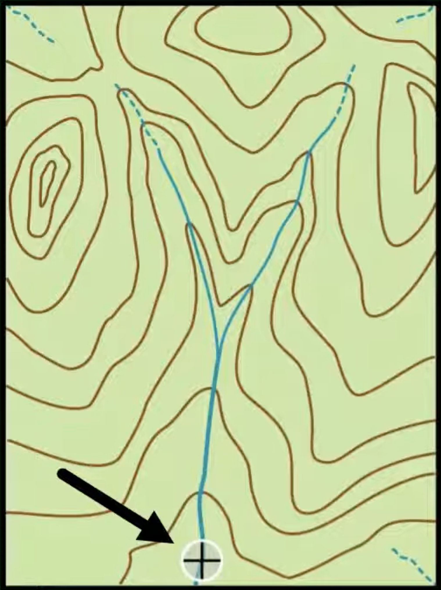
- Delineate the catchment boundary for the marked outlet.
- Now write down, as a numbered list, the procedure you actually followed. Aim for something around five steps, general enough that another student could apply it to a different map.
- Compare your procedure with those of two other groups. Where do they differ, and which of those differences are genuine disagreements rather than differences of wording?
- Justify two of your steps physically. Why must flow lines cross contours at right angles, and why must the boundary pass through high points and close on itself at the outlet?
- Identify the part of this map where you were least confident, and say why. More generally, what kinds of terrain make manual delineation unreliable?
- The surface catchment you have drawn need not be the groundwater catchment. Sketch a cross section showing how the two divides can separate, and give one practical consequence for water resource management.
- Finally, consider what is lost as well as gained when this task is handed to a computer. What are the limitations of manual delineation against digital, DEM-based methods, and what new problems does the digital approach introduce?
8. Water, climate and scarcity
Answer one of the following in about 400 words. These are the questions the textbook itself poses at the end of Chapter 1, and they are close in style to what you will meet in the exam.
(a) Discuss the physical properties of water, being hydrogen bonding, the density anomaly, specific heat capacity and latent heat, and explain how important each is in determining the natural climate of the Earth. Support your answer with numbers wherever you can.
(b) Consider the following statement:
“The total quantity of fresh water on earth could satisfy all the needs of the human population if it were evenly distributed and accessible.” — Stumm (1986: 201)
Evaluate it critically, drawing on the lecture and on Chapter 1. A strong answer will distinguish clearly between stores and fluxes, will give examples of spatial inequality in water resources, and will discuss how hydrology contributes to such problems both as a pure and as an applied science.
© How might water-poor countries overcome the lack of water resources within their borders? Consider abstraction, storage, transfers across borders, and trade in water-intensive goods, and say in each case where the problem has been moved to.